International Journal of Geosciences
Vol. 4 No. 8 (2013) , Article ID: 38632 , 7 pages DOI:10.4236/ijg.2013.48113
Modeling Near-Surface Air Temperature and Precipitation Using WRF with 5-km Resolution in the Northern Patagonia Icefield: A Pilot Simulation
1Dirección Meteorológica de Chile, Santiago, Chile
2Universidad de Magallanes, Punta Arenas, Chile
3GeoEstudios Ltda, Santiago, Chile
4Universidad de Chile, Santiago, Chile
Email: cvilla@meteochile.cl
Copyright © 2013 Claudia Villarroel et al. This is an open access article distributed under the Creative Commons Attribution License, which permits unrestricted use, distribution, and reproduction in any medium, provided the original work is properly cited.
Received July 15, 2013; revised August 17, 2013; accepted August 21, 2013
Keywords: Patagonia Ice Fields; WRF model; simulations
ABSTRACT
The regional Weather and Research Forecast (WRF) Model was run for the 2000-2010 period over the Northern Patagonia Icefield (NPI) with an horizontal resolution of 5 km. The regional model was initialized using the NCEP/NCAR atmospheric Reanalysis database. The simulation results, centered over the NPI, were validated against the observed data from the local surface stations in order to evaluate the improvement of the model results due to its increased horizontal resolution with respect to the lower resolution from Global Climate Model simulations. Interest in the NPI is due to 1) the large body of frozen water exposed to the impact of the warming planet, 2) the scarce availability of observed meteorological and glaciological information in this large and remote icefield, and 3) the need to validate the model behavior in simulating the current climate and its variability in complex terrain. The results will shed light on the degree of confidence in simulating future climate scenarios in the region and also in similar geographical settings. Based on this study subsequent model runs will allow to model future climate changes in Patagonia, which is basic information for estimating glacier variations to be expected during this century.
1. Introduction
General glacier retreat around the world is most likely responding to the global warming and contributing to the sea level rise as several studies indicate [1]. Those draining down from the Patagonian Ice Fields (PIF) show the same retreating behavior as respond to the environmental changes [2,3]. The PIF is located in the southern South America and it is part of the southward extension of the Andes Mountains. It is the largest temperate ice body of the world located in the extrapolar region in the Southern Hemisphere, covering an area of approximately 17,000 km2. The PIF is the most glaciated area of the Andes with several glaciers discharging into fiords on the ocean western side and into lakes on the continental eastern side. It is located in the midlatitudes being influenced by the Pacific Ocean and the westerly regime. The climate of the region is defined by the passing weather systems embedded in the westerly airflow and by the complex terrain.
The PIF is a relative narrow ice mass (10 - 50 km wide) oriented in a north-south direction and with elevations above 1500 m asl (above sea level). The ocean and the Patagonian steppe are only a few tens of kilometers to its western and eastern side, respectively. Both, the atmospheric and orographic factors result in a temperate and very humid environment in the western slope with annual accumulation reaching 5000 - 10,000 mm and less than 300 mm on the eastern slope [4-6]. In particular, the Northern Patagonian Icefield (NPI, Figure 1) covers an area about 3950 km2, from around 46˚31'S to 47˚45'W (this is about 138 km in a north-south direction) and has an ice thickness of 1460 ± 500 m [7]. The contribution of the NPI to the sea level rise accounted for about 27% of the total 0.042 ± 0.002 mm per year of the whole PIF during the period 1968/1975-2000 [2]. Therefore, defining the local and regional atmospheric environment is of relevant importance for cryospheric and biopheric studies, as well as for climate change and extreme hydro-mete-
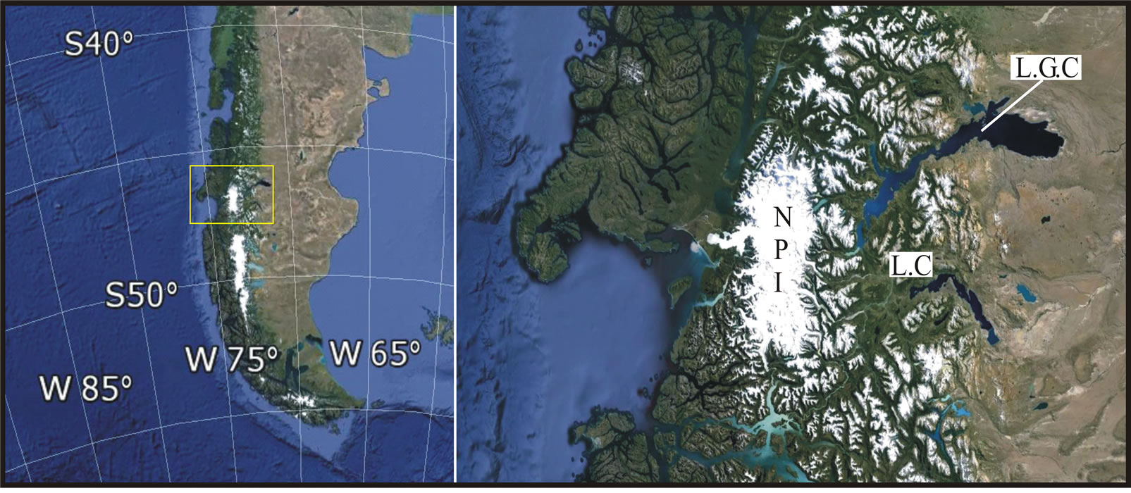
Figure 1. Location map of Southern South America and the Northern Pataganian Icefield (NPI). L.G.C. and L.C. identify the Lago General Carrera and Lago Cochrane, respectively.
orological events, in particular, the glacial lake outburst floods (GLOF) that can become of frequent occurrence in a warmer environment.
The availability of in-situ meteorological data is scarce in the region and numerical high-resolution simulations can be the option for providing the atmospheric data for meteorological and climate studies, but validation is necessary. Here, a validation of the numerical simulations at 5-km horizontal resolution, of the climate for 2000-2010 period obtained by the regional Weather and Research Forecast (WRF) model is presented. Application of the WRF model for simulating the present climate is the first effort of the Chilean Weather Service for subsequent simulation of present and future scenarios. The model results were validated by comparing the available observed data with the simulated data at closest gridpoint to the respective weather station (Table 1, Figure 2). Here, validation of the surface air temperature and precipitation as resolved by the model at 5-km resolution are presented.
2. Model Domains and Parameterizations
The WRF model was run for 11 years, from 2000 until 2010 centered over the NPI. The downscaling was done using the dynamic processes of the WRF model for three nested domains. The first was at 45-km, the second at 15-km and the third at 5-km horizontal resolution (Figure 3). The vertical resolution was 46 levels. The regional model domain 1 was initialized using the National Centers for Environmental Prediction (NCEP)-National Center for Atmospheric Research (NCAR), NCEP/ NCAR atmospheric Reanalysis database [8], which were available at global spatial resolution 2.5˚ × 2.5˚ lati-
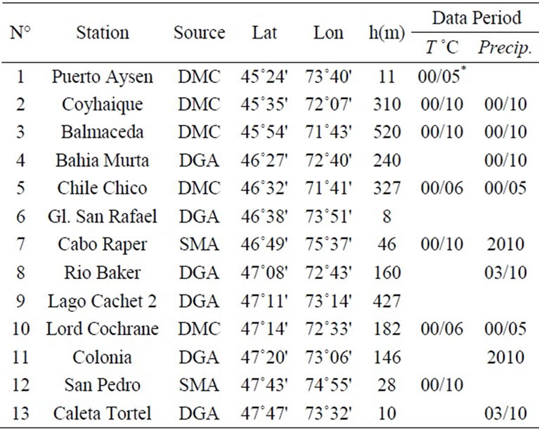
Table 1. List of weather stations.
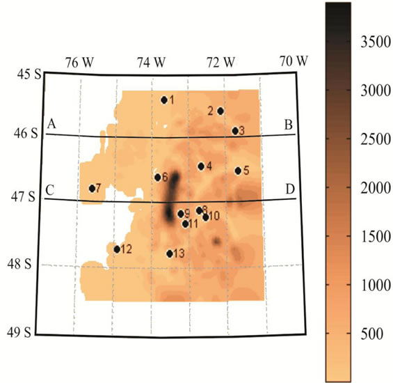
Figure 2. Geographical distribution of the weather stations listed in Table 1, along with the model elevation.
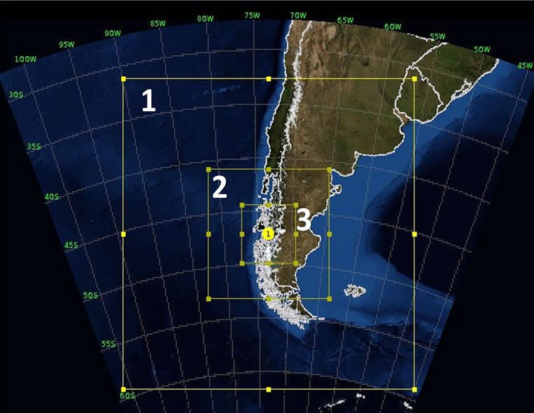
Figure 3. Regional model domains centered at NPI. Domain 1 is at 45-km, domain 2 at 15-km and domain 3 at 5-km horizontal resolution.
tude-longitude grids at standard pressure levels. The original time interval is 6 hours, from which daily and monthly averages were calculated. A complete description of the WRF for climate application can be found in Xin-Zhong et al. [9]. Some parameterizations included the physical scheme of Thompson et al. [10], the Rapid Radiative Transfer Model (RRTM) for longwave and shortwave radiation of Dudhia [11], the quasi-normal scale elimination (QNSE) surface layer, the QNSE boundary layer, the 5 layer thermal diffusion for land surface, the Betts-Miller-Janjic [12,13] schemes for cumulus and the operational ETA scheme.
The model was run on a Server computer AMD Opteron twelve core 6172 processor. One year simulation took around 12 integration computational days.
3. Results
3.1. Air Temperature
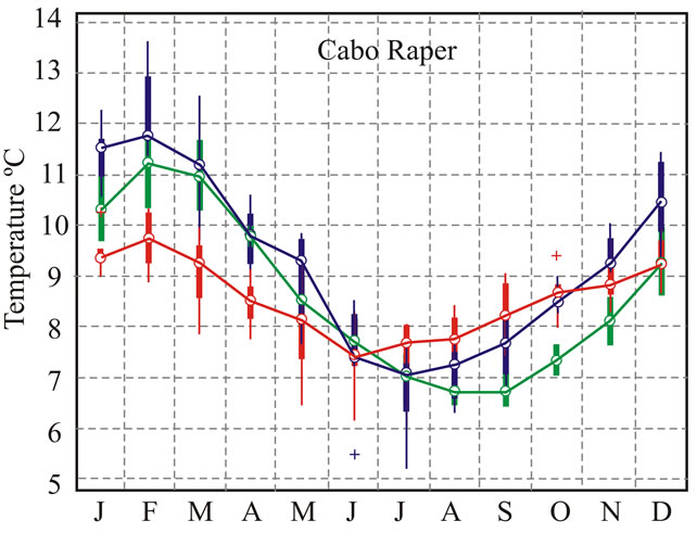
Overall, the model is able to simulate the annual cycle within the expected range of temperature values for the region. However, the seasonal behavior simulated by the model is lower than the observational data. Figure 4 compares the observed monthly mean air temperature registered at the coastal stations Cabo Raper (7) and San Pedro (12) and at the continental station Balmaceda (3), with the monthly mean as simulated by the model at the nearest grid-point from the respected stations. Results show that the model simulates colder temperatures for summer and warmer for winter months than the respect observed values.
Figure 4 also includes the monthly data from the NCEP/NCAR reanalysis from the closest grip-point at the weather station. Although the NCEP/NCAR results still show colder temperature in summer and spring in the two coastal stations; the seasonal behavior better agrees
 (a)
(a)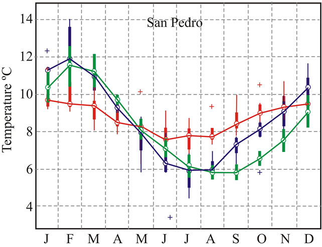 (b)
(b)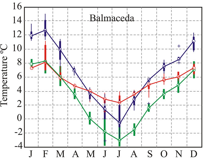 (c)
(c)
Figure 4. Observed (red) and simulated (blue) monthly mean (2001-2010) near-surface air temperature. (a) Cabo Raper (7); (b) San Pedro (12) and (c) Balmaceda (3). Blue: observed. Red: WRF simulation. Green: NCAR/NCEP Reanalysis.
with the observed monthly means than the WRF results. On the other hand, at the continental station Bal-maceda, the NCEP/NCAR monthly means show an overall colder environment year-round than the observed data. Comparing the monthly means obtained from the NCEP/ NCAR reanalysis with those from the WRF model, it can be seem that increasing the horizontal resolution flattens the annual cycle. In other words, WRF cools down (warms up) the warmer (colder) environment resolved by the NCEP/NCAR model. So that, WRF underestimates the annual cycle.
3.2. Precipitation
Model simulation overestimates the annual precipitation at Coyhaique (2) and Balmaceda (3) stations for about 200%, while it was only about 20% - 80% at Lord Cochrane (10) y Caleta Tortel (13) stations. The Root Mean Square Error (RMSE) analysis indicates that largest errors are found at Coyhaique, while in the other stations these errors are significant in summer and autumn. The correlation coefficient of the precipitation anomalies varies between 0.76 in Bahia Murta and 0.36 in Lord Cochrane (Figure 5). Despite of the important differences in the monthly precipitation, the annual and inter-annual variability are well simulated by the model (Figure 6).
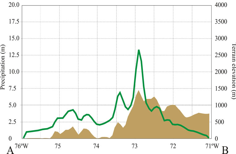
The vertical profiles at two selected latitudinal cross sections are displayed in Figure 7. The effect of the orography on the precipitation is clearly observed. The predominant windfield in this region is westerly. This results in larger accumulation on the western side than on the eastern side of the simulated mountains. The foehn effect on the lee side of the mountains implies that the precipitation rapidly decreases eastward. Therefore, precipitation is correlated with the terrain elevation (compare both
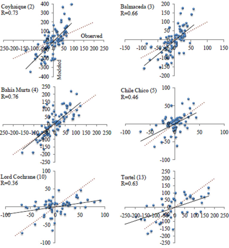
Figure 5. Correlation between the anomalies of the monthly precipitation registered by the weather stations and the accumulations simulated by the model at the respective nearby grid-points.
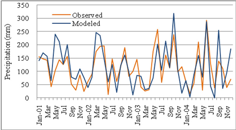
Figure 6. Monthly precipitation as simulated by the model domain 3 in Bahia Murta and the observed precipitation registered in the same place. The simulated curve was corrected for differences larger than 100 mm.
 (a)
(a)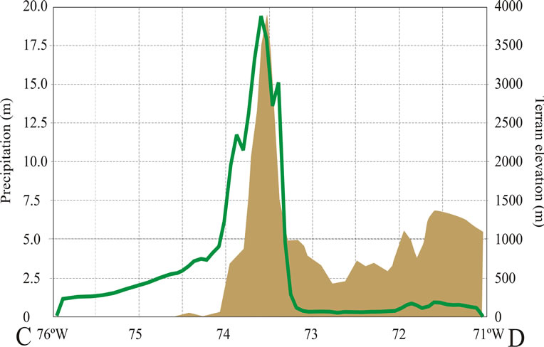 (b)
(b)
Figure 7. Latitudinal profile of the annual precipitation and terrain elevation simulated by the model at 46˚S (top) and at 47˚S (bottom).
profiles).
3.3. Spatial Simulation
Figure 8 shows the annual mean surface air temperature and annual mean precipitation accumulation fields in the region where the NPI is located. Left (right) panels are the near surface air temperature (mean annual precipita-
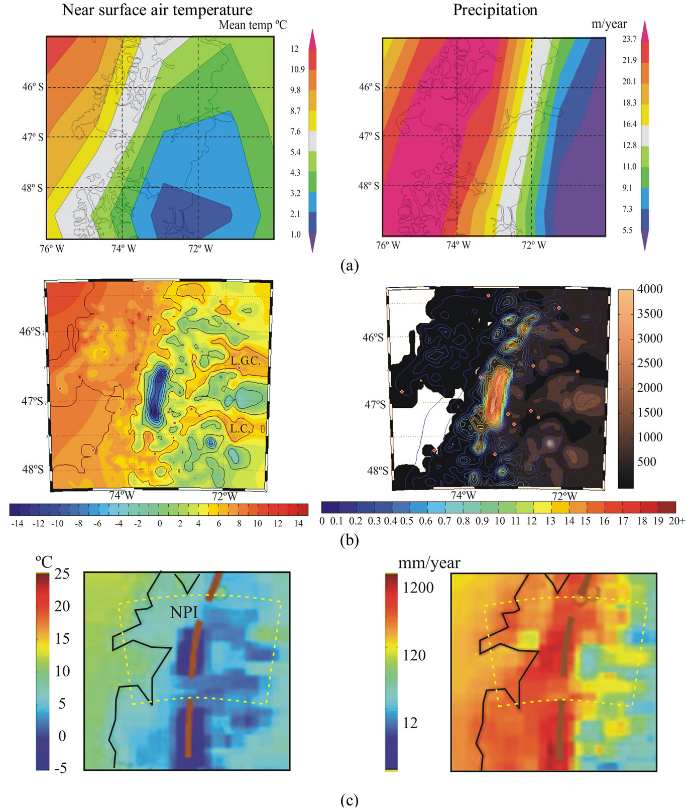
Figure 8. Model results from NCAR/NCEP R1 Reanalyses for annual mean air surface temperature and annual precipitation obtained (a), results from the WRF model at 5-km resolution (b), and the partial reproduction of the PRECIS-DGF regional model (c), where the precipitation scale is logarithmic. Yellow dashed lines inserted in the bottom panels approximately enclose the area simulated by the WFR model.
tion) simulations of the NCEP/NCAR reanalysis (top) obtained from the KNMI Climate Explorer website (http://climexp.knmi.nl) [14] for the 2000-2010 period, the simulation using the WRF model, domain 3 (middle) at 5-km grid-spacing resolution, and the partially reproduced simulation from the PRECIS-DGF model (bottom), run at 25-km resolution [5] for the 1978-2001 period. Even though, this latest model was run for different period, here is included for comparing the spatial resolution rather than actual values. Comparing the WRF model with both NCEP/NCAR reanalysis and PRECIS-DGF, it can be seen that the regional model resolved much more details than the other two, mainly with respect to the reanalysis field.
The NPI is relative well simulated with an area of air temperature below freezing. A distinct oval shape feature of air temperatures below 0˚C (light blue and blue colors) clearly identifies the NPI in the WRF simulation. Others areas of colder temperature can be associated with relative high elevations and ridges in the model terrain. Relative warmer air temperatures on the western side than on the eastern side of the NPI indicate that the model captures the influence of the ocean and continental effect. Also, the shapes of Lago General Carrera (L.G.C., or Lago Buenos Aires) and Lago Cochrane (L.C.) are simulated by the model. These features are not resolved by the NCEP/NCAR reanalysis, which in fact, simulated relatively warmer temperatures (above freezing values) in the interior of the continent, where supposedly the NPI is located. The PRECIS-DGF did resolve the NPI as an area of temperature below 0˚C, but less defined.
Also, the WRF simulation produces a more complex precipitation distribution (compare with both NCEP/ NCAR and PRECIS-DGF fields; right panels) where the topography plays an important role. The precipitation spatial distribution with increasing (decreasing) accumulation in the western (eastern) slope of the icefield is, as indicated earlier, the result of the orographic effect upon the westerly airflow (see right side panels). Eastward moving moist air masses are forced to rise up forming and/or enhancing the precipitation in the western side of the mountains, while descending airflow adiabatically dries the air masses inhibiting or decreasing the precipitation immediately eastward of the mountains ridge.
The WRF model better resolves the precipitation distribution than the NCEP/NCAR reanalysis and the PRECIS-DGF model. The precipitation on the NPI appears as the area of larger annual accumulation which can be above 14 m per year in high elevations. Similar result was found by Schaefer et al. [15] who used the same WFR model but for the 2005-2011 period. Note that the PRECIS-DGF model also resolved larger precipitation on the NPI region (same result is found with the WFR at 15 km horizontal resolution domain 2, not shown). This indicates that increasing the horizontal resolution implies better simulation of the precipitation, most probably due to the improving model topography.
The lack of in-situ weather stations precludes a complete validation of the simulated accumulations; however, estimations derived from river discharges [16], mass balance studies [17] and satellite-derived precipitation [18] suggest that accumulations of the order of 15 - 18 m per year are feasible. The precipitation reconstruction from varved sediments of Lago Plomo (around 47˚S) shows events above 15 m per year [19]. Shiraiwa et al. [20] found an accumulation of 17.8 m per year between the summers 1997/98 and 1998/99, but for Tyndall Glacier located in the southern SPI.
4. Conclusion
Here, we present the results of the surface air temperature and precipitation simulations using the WRF model, which was run for 2000-2010 period, using a nested computational grid with a high horizontal resolution of 5-km centered on the NPI. These results were compared with the available observational data, in order to validate the model, and how the increased resolution improves the model performance. Overall, the model simulated the seasonal behavior but with colder temperature during summer and warmer in winter. In other words, the model underestimated the annual cycle, mainly in the continental environment. On the other hand, the model overestimated the precipitation but captured the annual and inter-annual variability (Figure 6). The spatial distribution of the annual mean air temperature and precipitation shows details that are neither resolved by the NCEP/ NCAR reanalysis nor by the PRECIS-DGF simulations (at 25 km horizontal resolution). The pilot study reveals the advantages of improving the horizontal resolution of the regional model; for example, the model at 5-km resolution is able to better resolve details in the air temperature and precipitation distribution, just due to a better topography. However, the performance of the model regarding, for instance, with overestimation of the precipitation and underestimation of the annual cycle of the air temperature still need to be addressed.
5. Acknowledgements
This study is part of the Ice2Sea project funded by the EU 7 FP. Also, it was partially founded by the FONDECYT Project Nro 1090752. We thank to the Dirección Meteorológica de Chile, Dirección General de Aguas and the Servicio Meteorológico de la Armada for the weather data.
REFERENCES
- P. Lemke, J. Ren, R.B. Alley, I. Allison, J. Carrasco, G. Flato, Y. Fujii, G. Kaser, P. Mote, R. H. Thomas and T. Zhang, “Observations: Changes in Snow, Ice and Frozen Ground,” In: S. Solomon, D. Qin, M. Manning, Z. Chen, M. Marquis, K. B. Averyt, M. Tignor and H. L. Miller, Eds., Climate Change 2007: The Physical Science Basis. Contribution of Working Group I to the Fourth Assessment Report of the Intergovernmental Panel on Climate Change, Cambridge University Press, Cambridge, New York, 2007.
- E. Rignot, A. Rivera and G. Casassa, “Contribution of the Patagonia Icefields of South America to Sea Level Rise,” Science, Vol. 302, No. 5644, 2003, pp. 434-437. http://dx.doi.org/10.1126/science.1087393
- P. López and G. Casassa, “Recent Acceleration of Ice Loss in the Northern Patagonia Icefield Based on an Updated Decennial Evolution,” The Cryosphere Discuss, Vol. 5, No. 6, 2011, pp. 3323-3381. http://dx.doi.org/10.5194/tcd-5-3323-2011
- J. F. Carrasco, G. Casassa and A. Rivera, “Meteorological and Climatological Aspects of the Southern Patagonia Icecap,” In: G. Casassa, F. V. Sepúlveda and R. M. Sinclair, Eds., The Patagonian Icefields: A Unique Natural Laboratory for Environmental and Climate Studies, Kluwer Academic, Boston, 2002, pp. 29-41. http://dx.doi.org/10.1007/978-1-4615-0645-4_4
- R. Garreaud, P. Lopez, M. Minvielle and M. Rojas, “Large-Scale Control on the Patagonian Climate,” Journal of Climate, Vol. 26, No. 1, 2013, pp. 215-230. http://dx.doi.org/10.1175/JCLI-D-12-00001.1
- J.-C. Aravena and B. H. Luckman, “Spatio-Temporal Rainfall Patterns in Southern South America,” International Journal of Climatology, Vol. 29, No. 14, 2009, pp. 2106-2120. http://dx.doi.org/10.1002/joc.1761
- G. Casassa, “Ice Thickness Deduced from Gravity Anomalies on Soler Glacier, Nef Glacier and the Northern Patagonia Icefield,” Bulletin of Glacier Research, Vol. 4, 1987, pp. 43-57.
- E. M. Kalnay, et al., “The NCEP/NCAR 40-Year Reanalysis Project,” Bulletin American Meteorological Society, Vol. 7, 1996, pp. 437-471. http://dx.doi.org/10.1175/1520-0477(1996)077<0437:TNYRP>2.0.CO;2
- X.-Z. Liang, et al., “Regional Climate-Weather Research and Forecasting Model,” Bulletin of American Meteorological Society, Vol. 93, No. 9, 2012, pp. 1363-1387. http://dx.doi.org/10.1175/BAMS-D-11-00180.1
- G. Thompson, P. R. Field, R. M. Rasmussen and W. D. Hall, “Explicit Forecasts of Winter Precipitation Using an Improved Bulk Microphysics Scheme. Part II: Implementation of a New Snow Parameterization,” Monthly Weather Review, Vol. 136, No. 12, 2008, pp. 5095-5115. http://dx.doi.org/10.1175/2008MWR2387.1
- J. Dudhia, “Numerical Study of Convection Observed during Winter Monsoon Experiment Using a Mesoscale Two-Dimensional Model,” Journal of Atmospheric Science, Vol. 46, No. 20, 1989, pp. 3077-3107. http://dx.doi.org/10.1175/1520-0469(1989)046<3077:NSOCOD>2.0.CO;2
- A. K. Betts and M. J. Miller, “A New Convective Adjustment Scheme. Part II: Single Column Tests Using GATE Wave, BOMEX, ATEX and Arctic Air-Mass Data Sets,” Quarterly Journal of the Royal Meteorological Society, Vol. 112, No. 473, 1986, pp. 693-709.
- Z. L. Janjic, “The Step-Mountain Eta Coordinate Model: Further Developments of the Convection, Viscous Sublayer and Turbulence Closure Schemes,” Monthly Weather Review, Vol. 122, No. 5, 1994, pp. 927-945. http://dx.doi.org/10.1175/1520-0493(1994)122<0927:TSMECM>2.0.CO;2
- G. J. van Oldenborgh, S. S. Drijfhout, A. van Ulden, R. Haarsma, A. Sterl, C. Severijns, W. Hazeleger and H. Dijkstra, “Western Europe Is Warming Much Faster than Expected,” Climate of the Past, Vol. 5, No. 1, 2009, pp. 1-12. http://dx.doi.org/10.5194/cp-5-1-2009
- M. Schaefer, H. Marchguth, M. Falvey and G. Casassa, “Modeling Past and Future Surface Mass Balance of the Northern Patagonia Icefield,” Journal of Geophysical Research, Vol. 118, No. 2, 2013, pp. 571-588. http://dx.doi.org/10.1002/jgrf.20038
- F. Escobar, F. Vidal and C. Garin, “Water Balance in the Patagonia Icefield,” In: R. Naruse, Ed., Glaciological Researches in Patagonia, Japanese Society of Snow and Ice, 1992, pp. 109-119.
- E. Rignot, A. Rivera and G. Casassa, “Contribution of the Patagonia Icefields of South America to Sea Level Rise,” Science, Vol. 302, No. 5644, 2003, pp. 434-437. http://dx.doi.org/10.1002/jgrf.20038
- M. Falvey and R. D. Garreaud, “Wintertime Precipitation Episodes in Central Chile: Associated Meteorological Conditions and Orographic Influences,” Journal of Hydrometeorology, Vol. 8, No. 2, 2007, pp. 171-193. http://dx.doi.org/10.1175/JHM562.1
- J. Elbert, M. Grosjean, L. von Gunten, R. Urrutia, D. Fischer, R. Wartenburger, D. Ariztegui, M. Fujak and Y. Hamann, “Quantitative High-Resolution Winter (JJA) Precipitation Reconstruction from Varved Sediments of Lago Plomo 47˚S, Patagonian Andes, AD 1530-2002,” The Holocene, Vol. 22, No. 4, 2011, pp. 465-474. http://dx.doi.org/10.1177/0959683611425547
- T. Shiraiwa, S. Kohshima, R, Uemura, N. Yoshida, S. Matoba, J. Uetake and M. Godoi, “High Net Accumulation Rates at Campos de Hielo Patagónico Sur, South America Revealed by Analysis of a 45.97 m Long Ice Core,” Annals of Glaciology, Vol. 35, No. 1, 2002, pp. 84-90. http://dx.doi.org/10.3189/172756402781816942