Journal of Financial Risk Management
Vol.04 No.03(2015), Article ID:60111,22 pages
10.4236/jfrm.2015.43018
Granular and Star-Shaped Price Systems
Erio Castagnoli1, Marzia De Donno2, Gino Favero2, Paola Modesti2*
1Accademia Nazionale Virgiliana and Università Bocconi, Mantova and Milan, Italy
2Università degli Studi di Parma Dipartimento di Economia, Parma, Italy
Email: *paola.modesti@unipr.it
Copyright © 2015 by authors and Scientific Research Publishing Inc.
This work is licensed under the Creative Commons Attribution International License (CC BY).
http://creativecommons.org/licenses/by/4.0/


Received 17 July 2015; accepted 27 September 2015; published 30 September 2015
ABSTRACT
Linear price systems, typically used to model “perfect” markets, are widely known not to accommodate most of the typical frictions featured in “actual” ones. Since some years, “proportional” frictions (taxes, bid-ask spreads, and so on) are modeled by means of sublinear price functionals, which proved to give a more “realistic” description. In this paper, we want to introduce two more classes of functionals, not yet widely used in Mathematical Finance, which provide a further improvement and an even closer adherence to actual markets, namely the class of granular functionals, obtained when the unit prices of traded assets are increasing w.r.t. the traded amount; and the class of star-shaped functionals, obtained when the average unit prices of traded assets are increasing w.r.t. the traded amount. A characterisation of such functionals, together with their relationships with arbitrages and other (more significant) market inefficiencies, is explored.
Keywords:
Arbitrage, Asset Pricing, Super-Hedging, Granularity, Star-Shaped Prices

1. Introduction
One of the first and biggest concerns of Mathematical Finance is to study the prices of a suitable set of risky financial assets of any type, including stocks, indexed bonds, variable rate deposits, derivative securities, and so on. Usually, financial assets are modeled as random variables on some state sets, which are supposed to be the same for every asset in the considered market.
In earlier models, such as the one leading to the celebrated Black, Scholes, and Merton formula for option pricing ( Black & Scholes, 1973 ; Merton, 1973 ), the market is supposed to be a perfect one; in particular, no frictions are featured and no bid-ask spreads or commissions affect prices. Consequently, as it is clearly shown, for instance, in Dothan (1990) , Pliska (1997) , and Björk (1999) , asset prices turn out to be linear with respect to assets themselves, in the sense that the price of the sum of two positions exactly equals the sum of the two separated prices. In such a setting, a central result is found, called the Fundamental Theorem of Asset Pricing, of which dozens of variants are featured in the literature (besides the cited books see, for instance, Delbaen & Schachermayer, 1994 , for quite a general version), which essentially is a representation theorem: roughly speaking, the market prices do not allow for arbitrages (i.e., free gains without risks) if and only if there exist a probability measure called the risk neutral probability―and a discount factor such that prices themselves are (discounted) expected values of the future asset values.
The perfect market model, however, quickly proves to be unfit to provide a good description of realistic markets. For instance, it may be impossible to obtain the exact replication of a given pay-off, and therefore no linear price can be given for it. In such a case, as investigated by Davis & Clark (1994) , the investor may naturally aim at super-hedging it, i.e., at getting at least as much as needed (possibly more) at the minimum possible price. There are also cases when, due to market frictions, a dynamical strategy that exactly replicates the given pay-off may turn out to be more expensive than a super-hedging one: see, e.g., Hodges & Neuberger (1989) . El Karoui & Quenez (1995), Jouini & Kallal (1995), Jouini (1997), and Cvitanić et al. (1999) among others, had investigated such a setting and found a representation theorem: in any case, super-hedging prices turn out to be the maximum of a family of linear prices, which, for instance, Cvitanić et al. (1999) interpreted as prices in “shadow markets”. Moreover, Pham (2000) studied the properties of super-hedging price functionals to find them sublinear: additivity was replaced by subadditivity, meaning that the price of the sum of two positions might be cheaper than the sum of the two separated prices. Since sublinearity entails positive homogeneity besides subadditivity, it turns out to be perfectly fit to describe markets affected by proportional transaction costs (such as taxes or percentage commissions): see, e.g., Pham, Touzi, & Touzi (1999) . Furthermore, sublinearity turned out to be interesting for risk management purposes as well, being the foundational point for the celebrated paper by Artzner et al. (1999) on coherent risk measures.
A class of risk measures more general than the sublinear (i.e., coherent) ones of Artzner et al. (1999) is proposed by Föllmer & Schied (2002) , who replace sublinearity with the weaker convexity1. Inspired by their work, we started wondering whether convex price functions may sensibly be adapted to financial markets: we realized that this was naturally the case, for instance, if unit asset prices are supposed to increase with respect to the traded amount. A representation result can be found, stating that convex price functionals are the upper envelope of a family of affine prices, which admit an interpretation similar to the “shadow markets” of Cvitanić et al. (1999) .
Another, further generalisation, may require average unit asset prices to be increasing, instead of “marginal” ones. This may be the case, for instance, when an agent can choose to buy an asset on several different markets, featuring different increasing unit prices: of course, the purchase will be conducted in such a way that the overall price (or, which is the same, the average unit price) is as low as possible. This leads to a totally new class of price functions, which we name star-shaped because their epigraph turns out to be a star-shaped set with respect to the origin, in the sense of Stewart & Tall (1983) . A representation result can be given for this class of functionals as well, with an interesting economical interpretation.
In the remaining part of this section, the notation used throughout the entire paper is stated, and the current state of the literature about linear and sublinear prices is briefly summarized. Although in different notation, everything exposed here can be found, for instance, in Dothan (1990) , Pliska (1997) , and Björk (1999) for the linear setting, and in Jouini & Kallal (1995) and Koehl & Pham (2000) for the sublinear case. Some examples, in a simple discrete setting, are also given, in order to allow the reader for familiarising with the phenomena under study. Remarkably, we emphasise that, as soon as the price functional is no longer linear, market efficiency is no longer guaranteed by absence of arbitrages only, and that another class of inefficiencies, namely the convenient super-hedgings (roughly speaking, the opportunity to get a better pay-off at a lower price), have to be taken into account.
Section 2 is dedicated to introducing and examining the convex case. After observing that convex functions naturally pop out when pricing by super-hedging by means of assets whose unit price is increasing, we give a generalisation of the Fundamental Theorem of Asset Pricing, and give an interpretation of the representation in terms of market efficiency. It turns out that the market is fully efficient, i.e., that no convenient super-hedging is possible, if all of the “shadow markets” are efficient, whereas absence of arbitrage is guaranteed by a local, less restrictive property.
Star-shaped prices are analysed in Section 3. We show that such functionals are the result of pricing by super- hedging by means of assets whose average price is increasing, and show that such a requirement is actually a proper generalisation of the previous, convex case. We also introduce a new pricing technique, which we may call “super-hedging by chunks” and that mathematically corresponds to the inf-convolution of the price functionals of the “shadow markets”. We show that convexity and star-shape are in some sense “stable” under super-hedging, either in the classical sense or in the “by chunks” one, and analyse the representation of star-shaped functionals in terms of market efficiency.
Finally, Section 4 is dedicated to summarising and comparing the main properties and the efficiency conditions of the four analysed market types and Section 5 features some concluding remarks.
1.1. Notation
A state space
 is supposed to be given, and the market
 is a set of (real valued) random variables2
 : every
 is identified with an asset, in the sense that the (random) value attained by X corresponds to the pay-off (or the market value) of the considered asset at a suitable maturity. We are supposing that the uncertainty is resolved in a single time period: in other words, the models we encompass are of a static, not dynamic, type. We write
 (respectively,
 ) to intend that
 (respectively,
 ) for every
 , where
 indicates the usual weak inequality between real numbers.
We shall suppose one of the classical “perfect market hypotheses” to hold, requiring every asset
 to be infinitely available (there is no “maximum tradable amount”) and divisible (it is possible to buy any fraction of it); furthermore, short sales are allowed. This translates into the fact that, for every
 and every
 , the investor can hold the position
 (where
 indicates short sale of
 units of X). Of course, several assets
 can be simultaneously traded, by buying
 units of each (with
 indicating short sale); this corresponds to holding a portfolio of those n assets, whose “final” pay-off plainly turns out to be
 . Mathematically speaking, this corresponds to
 being a linear space.
Giving a price to every traded asset
 simply amounts to defining a (price) functional
 . The functional
 is said to allow for:
• An arbitrage (see, e.g.,
Björk, 1999
and
Pliska, 1997
) if there exist a
 in
in
 such that
 (which means that it is possible to obtain an immediate gain, corresponding to the negative price, without any risk, i.e., with the certainty not to lose any money at the maturity);
• A convenient super-hedging (quite a recent concept: see, e.g.,
Castagnoli et al., 2009
and
Castagnoli et al., 2011
, but also, for instance,
Hodges & Neuberger (1989)
, who observe the phenomenon although without specifically titling it) if there exist
 such that
 and
and
 (which means that it is possible to obtain a “higher” pay-off at a “lower” price).
Of course, the basic laws of supply and demand imply that neither of the above opportunities, which we shall jointly refer to as inefficiencies, should hold in a market: in both cases, the demand pressure on X would quickly lead its price
 to increase until becoming either positive (in the first case) or greater than
 (in the second case; furthermore, lack of demand on Y would lead its price
 to decrease as well). Note that:
•
 does not allow for arbitrages if and only if
 whenever
 , that is, if
 is (or may be called) positive;
•
 does not allow for convenient super-hedgings if and only if
 whenever
 , that is, if
 is (or may be called) increasing.
Generally speaking, absence of arbitrages has the nature of a local property, because it only involves the behaviour of the price functional
 with respect to the null pay-off, whereas absence of convenient super-hedgings is a global property, because it is required to hold for every pair
 .
.
It is noteworthy as well that there are no general links between positivity and monotonicity. Take for instance, : the functional
 is (of course) positive but not increasing (because, taken a
 in
in , it is
 and
and ), whereas, taken a
 in
in , the functional
 is increasing but
not positive (because , although
 ).
).
Note also that, for every , the price functional
 induces a function
 defined by
 , which in a natural way can be called the supply and demand function for X.
Remark 1. We purposefully decided to avoid measurability issues: in particular, we never mentioned the ( -)algebra
 on
on
 where the probability P is properly defined (and with respect to which all the
 have to be measurable). This is only possible because of our choice of dealing with single period models: in order to introduce a dependence from time, actually, it is unavoidable to follow the well-known approach of defining a filtration
 of (
of ( -)algebrae contained in
 and to suppose that, at every time
 , the value (price) of a random variable
 is given by its conditional expected value
 , possibly discounted in a suitable way.
In the same way, the price functional
 should be taken to be measurable with respect to the (
 -)algebra
 (and the Borel
 -algebra
 on
on ). As a matter of fact, the most general setting for this situation is to take an arbitrary (real) linear space
 and to consider as possible price functionals all of the elements of a subspace
 of the algebraic dual of
 . Moreover, by considering on
 the weak topology (i.e., the minimal one that makes continuous all of the
 ),
),
 turns out to be the topological dual of
 , so that our setting can be included in the topological duality among linear spaces, a typical topic in Functional Analysis. Some more details can be found in
Castagnoli et al. (in print)
and references therein.
, so that our setting can be included in the topological duality among linear spaces, a typical topic in Functional Analysis. Some more details can be found in
Castagnoli et al. (in print)
and references therein.
Remark 2. The arbitrage and convenient super-hedging opportunities defined above are often called strong in the literature, and their weak counterparts are defined as follows. Write
 to indicate that
 and
and
 (that is, there exists at least an
 such that
 ). In such a case, the functional
 is said to allow for:
• A weak arbitrage (or an arbitrage of the second kind) if there exists a
 in
in
 such that
 (the case
 is allowed, possibly cancelling the immediate gain, but in some states a gain at the maturity will be obtained);
• A weak convenient super-hedging (or a convenient super-hedging of the second kind) if there exist
 such that
 and
and
 (the prices may coincide, but in some states X will pay off strictly better than
 ).
).
It is straightforward that:
•
 does not allow for weak arbitrages if and only if
 whenever
 : that is, if and only if
 is strictly positive;
•
 does not allow for weak convenient super-hedgings if and only if
 whenever
 : that is, if and only if
 is strictly increasing.
As a matter of fact, when the assets
 are not discrete random variables, the above definitions turn out to be impossible to deal with (they would imply, for instance, that for every
 the “Dirac function”
 gets a positive price
 , which is plainly meaningless). It is then customary to take into consideration an a-priori probability P on
 , and to define
 when
when
 and
and . In such a case, all of the “inequalities” between random variables are of course to be intended in the “P-almost everywhere” sense.
We decided not to take into consideration the weak arbitrages, both for the sake of simplicity and because we want to emphasize that there is no actual need for the a priori probability P to be given. It is nevertheless proper to cite this cases, both for compatibility with the existing literature and to remark that asking for weaker and weaker inefficiencies to be removed from the market translates into stronger and stronger regularity properties for the price functional .
.
It is also noteworthy that, in order to define weak inefficiencies and to intend the inequalities “almost everywhere”, instead of an a priori probability P, any a priori measure
 equivalent to P could be considered on
 : it would actually be exactly the same to define
 whenever
 and
and , i.e., when the set where
 has a positive measure instead of a positive probability. Briefly said, the normalisation property of the a priori measure is completely unnecessary.
1.2. Perfect Markets: The Linear Case
Besides the infinite availability and divisibility hypotheses cited above, the classical models based on “perfect markets” (see the already cited Björk, 1999 , Pliska, 1997 , and Dothan, 1990 ) ask for three more requirements. First of all, all market agents are fully rational and they aim at maximising their profit; furthermore, all agents are equally informed, without “informational asymmetries”. Secondly, the agents are price takers: they have no possibility to negotiate the prices they see on the markets. Finally, in the market there are no taxes, no bid-ask spreads, no commissions: in a word, there are no frictions.
All of these hypotheses together could be simply summarised in a single property: a market is called perfect if the price functional
 is linear. Recall that the linearity of
 means that
 for every
 and every
 ; equivalently,
 is additive (
 for every
 ) and homogeneous (
 for every
 and every
 ). Note that this translates into the fact that the unit price for every asset
 does not depend on the traded amount: buying (or short selling) a units of X exactly costs (or yields)
 times the unit price of X. In other words, the supply and demand function
 is a linear function for every
 : for every
 ,
, .
.
Every linear functional on a linear space attains null value at the “origin” (i.e., at the null vector): as an immediate consequence, an increasing linear functional turns out to be positive as well. Shortly said, for linear functionals, (increasing) monotonicity implies positivity. In the case of linear functionals, moreover, the converse is also true:
 is equivalent to
 , and the fact that
 immediately yields that a positive linear functional is increasing as well. In other words, positivity and monotonicity are equivalent in the linear setting: therefore, in the classical literature about perfect markets, convenient super-hedgings have never been specifically recognised as market inefficiencies, because a price functional allows for convenient super-hedgings if and only if it allows for arbitrages.
A classical duality result states that, given a linear space
 of real valued functions defined on the same set
 , a functional
 is linear if and only if there exist a (signed) measure
 on
on
 such that

(Lebesgue integrals). Usually, it is said that
 can be represented as the Lebesgue integral with respect to a suitable measure
 defined on
 ; we remark that the measure
 may be “signed”, i.e., that it may attain negative values. The Fundamental Theorem of Asset Pricing, translated into our setting, states that the price functional
 allows for no arbitrages if and only if it is represented by a “proper” positive measure
 .
.
If the “constant” (degenerate) random variables
 belong to
 (or, equivalently, if the monetary unit
 belongs to
 ), then the price of
 amounts to
 : in other words, the “norma-
lisation factor”
 has the financial meaning of the discount factor for the considered time period. Note also that the measure
 turns out to be a probability on
 : this way, the above representation of the price functional becomes
 (1)
(1)
which is classically told by stating that, if no arbitrages are allowed, the current prices of financial assets are the discounted expected values of their final random pay-off. In such a case,
 is called a risk-neutral probability (or, in the dynamical case, a martingale measure).
Example 1. Take into consideration the state space : since
 is finite, every random variable
 can be identified with the vector
 : therefore, we shall simply write
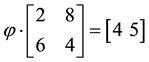
 . Suppose that two assets are exchanged on the market:
 , at price 4, and
 , at price 5.
The decision to hold a portfolio obtained by buying (or short selling)
 units of
 and
and
 units of

 can be identified with the vector
 : it leads to the pay-off
 and costs
 . Note that every pay-off
 can be obtained by means of a suitable (and unique) portfolio: in other
words,
 , where it is intended that the price of every
 is defined as the price of the portfolio a yielding the pay-off X.
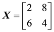
We can simplify the notation by defining the pay-off matrix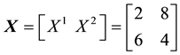 : this way, the portfolio
 simply leads to the pay-off
 (usual matrix product). If we further define the price vector
 , it is clear that the price of the portfolio a is
 .
.
Note that every linear functional
 simply amounts to the vector (“inner”) product by a vector
 , with
 and
and : indeed,
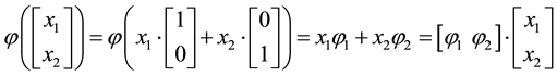 .
.
Let us now represent the price functional . As we already mentioned, for every
 it has to be
 , with a such that
 . Suppose now that
 is a vector such that
 :3 it is immediate
that , and therefore that
 represents
 . Since the linear system
 has
has
the unique solution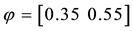 , such a vector turns out to be the representation of the linear price functional
 induced by the market prices.
It is immediate to realise that, since both components of
 are positive, the functional
 is (positive, and therefore) monotonically increasing. This shows that no arbitrages are allowed in the market. Note also that the
discount factor is , and that the vector
 corresponds to a probability Q on
 , assigning
 ,
, . Furthermore, for every
 ,
, .
.
Just for the sake of completeness, suppose that the price of
 be 8 instead of 4. In this case, the unique so-
lution of the system
 would be
 the presence of a non-positive component implies that
 is not positive and that indicates the possibility of arbitrages. Indeed, the pay-off
 is obtained with the portfolio
 at the price
 .
.
1.3. Proportional Frictions: The Sublinear Case
A natural generalisation of the linear model is to suppose that some frictions affect the market, in order to accommodate, for instance, taxes or commissions. By supposing such frictions to be proportional to the traded amount, it is possible to maintain “half” of the homogeneity property of the price functional: namely,
 turns out to be positively homogeneous, meaning that
 for every
 and every
 (no longer for every
 ).
).
It is clear that such a price functional can no longer be expected to be additive: for instance, an agent buying both
 and
and
 will pay the taxes and commissions on both of them, and thus will end up paying a positive price for the null pay-off: in symbols,
 . Nevertheless, since the agents are still supposed to be rational, it is reasonable to suppose that
 is subadditive, i.e., that
 (if the price of a joint position were greater than the sum of the two composing ones, every rational agent would separately buy the two components).
If , generally speaking, the bid price induced by a pricing functional is
 . If
. If
 is (sublinear, and therefore) subadditive, recalling that
 , we get
 , where we write
 to underline that those expressed by
 actually are ask prices. Roughly speaking, then, sublinear functionals model the case when the ask and the bid price may differ (due to taxes, commissions, or general bid-ask spreads), yet the unit price does not depend on the traded amount. The supply and demand function induced by a sublinear
 for a given
 takes the form
 .
.
Every sublinear functional attains null value at the origin: therefore, every increasing sublinear functional is positive as well. The converse is not true, as already mentioned: the norm functional is positive, but not increasing. As a consequence, there may be sublinear price functionals that allow for convenient super-hedgings although not allowing for arbitrages. It is noteworthy, nevertheless, that
 turns out to be increasing every time that it is “negative”, i.e., when
 for every
 : in such a case, indeed, whenever
 we get
 . Recalling that the bid price of the pay-off X is naturally defined as
 , the “negativity” condition translates into
 for every
 : in other words, absence of arbitrages is guaranteed by the positivity of ask prices of the positive pay-offs, whereas absence of convenient super-hedgings is ensured by the positivity of bid prices of the same positive pay-offs.
As an immediate consequence of the classical Hahn-Banach Theorem, a sublinear functional
 can be represented as the pointwise maximum of the linear functionals that it “dominates”. In greater detail: if
 is a sublinear functional, then the set
 is not empty and
 . Moreover, if
 is not allowed to take infinite values, L turns out to be convex and compact, so that the “sup “can be replaced by a “max”. It is possible to show (see
Pliska, 1997
and
Castagnoli et al., 2009
) that:
is not allowed to take infinite values, L turns out to be convex and compact, so that the “sup “can be replaced by a “max”. It is possible to show (see
Pliska, 1997
and
Castagnoli et al., 2009
) that:
•
 is positive if and only if there exists (at least) a positive
 ;
;
•
 is increasing if and only if every
 is positive.
From a mathematical point of view, L is the subdifferential of
 at 0 (see, e.g.,
Rockafellar, 1970
).
at 0 (see, e.g.,
Rockafellar, 1970
).
According to such a characterisation, if
 does not allow for convenient super-hedgings (and, therefore, not even for arbitrages), every
 can be represented as the expected value with respect to a suitable measure
 , discounted by a suitable factor
 :
:

In other words, an efficient sublinear functional acts “as if” a whole set L of “plausible” scenarios
 are involved, each corresponding to (a linear price functional, i.e., to) a probability measure
 and a discount factor
 : the price assigned to every random variable amounts to the “worst case” discounted expected value, i.e., to the linear functional assigning the highest price to X. It is noteworthy to mention that such a representation was already conjectured by
de Finetti & Obry (1933)
.
: the price assigned to every random variable amounts to the “worst case” discounted expected value, i.e., to the linear functional assigning the highest price to X. It is noteworthy to mention that such a representation was already conjectured by
de Finetti & Obry (1933)
.
One final consideration is in order. A rational investor who aims at obtaining the pay-off
 (which need not belong to
 ) is naturally led to look for the best (super)hedge of Z, i.e., to buy the cheapest traded asset
 that dominates Z
(El Karoui & Quenez, 1995)
. This way, (a better pay-off than) Z can be obtained at the price
that dominates Z
(El Karoui & Quenez, 1995)
. This way, (a better pay-off than) Z can be obtained at the price
called the cheapest super-hedging price of Z. It is quite clear that, if
 does not allow for convenient super-hedgings,
 for every
 ; on the other hand, it is immediate to realise that, if
 allows for convenient super-hedgings, then
 . It is indeed possible to show that
 is sublinear as soon as
 is and that, if
 , then
 with
with .
.
Roughly speaking,
 turns out to be the highest sublinear functional, among those dominated by
 , that does not allow for (arbitrages or) convenient super-hedgings.
Example 2. Consider the same two assets of Example 1, with pay-off matrix , but suppose now
that two price vectors are given, namely that of the ask prices
 and of the bid prices
 (of course
 ). The price of every
 is found as its cheapest super-hedging price:
 (where
 and
and

denote the positive and negative part of
 respectively). A standard linear programming duality argument4 allows to conclude that the price
 dominates the linear functional induced by the vector
 if and only if
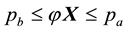 , which amounts to finding all the js such that
 , with
 .
.
The solutions of the given parametric linear system is the set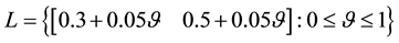 : it is immediate to check that it is a convex and compact subset of
 . Since L contains positive vectors only, we can conclude that
 allows for no convenient super-hedgings (and, therefore, for no arbitrages).
It is possible to build examples when the functional
 induced by the listed assets allows for arbitrages and for convenient super-hedgings, or for convenient super-hedgings only. For the sake of brevity, we invite the interested reader to see
Castagnoli et al. (2009)
.5
induced by the listed assets allows for arbitrages and for convenient super-hedgings, or for convenient super-hedgings only. For the sake of brevity, we invite the interested reader to see
Castagnoli et al. (2009)
.5
2. Increasing Unit Prices
The Granular (Convex) Case
Although sublinear prices can indeed capture several features of prices in the “real world”, they still feature unit prices which do not depend on the traded amount. Who trades on actual markets, instead, knows well that unit prices tend to increase with respect to the amount bought, and to decrease with respect to the amount sold. Suppose, for instance, that we are set to buy 1000 units of some asset. Having a look at the offer prices, we see that someone is selling up to 100 units at 3?each, someone else up to 500 units at 3.1?each, someone else up to 600 units at 3.2?each, and so on. This way, we are facing increasing unit prices, and to buy all of the 1000 units we have to pay : it is immediate to realise that, generally speaking, total price needed to buy
 units of an asset turns out to be a(n increasing and) convex function of
 (and piecewise affine, in our example, but this is not necessary: the price is a convex function of the traded amount every time that the marginal price is increasing, which is the standard hypothesis of the classical law of supply and demand). We want to show that a natural way to model such a situation is to take into consideration a convex price functional
 (which is of course a generalisation of the sublinear case, because every sublinear functional is convex as well): in order to do so, let us see how a convex price functional comes out in a very natural way.
Suppose that, in an exchange list under consideration, the assets
 are included, such that, for every
 , the supply and demand function
 is increasing and convex. Of course, the set
 of all attainable pay-offs is the linear space spanned by the traded assets:
 . The only reasonable way of assigning a price to every
 is to use the super-hedging technique seen at the end of the previous section:
It is immediate to show that such functional
 is increasing5; since
 , the monotonicity of
 implies its positivity, which, from the financial point of view, means that the “cheapest super-hedging” price functional
 does not allow neither for arbitrages nor for convenient super-hedgings. It is also possible, although a little technical, to show that
 is convex, i.e., that
 for every
 and every
 6: the convexity of the single supply and demand functions “propagates” to the entire pricing functional.
Fenchel’s Theorem ensures that a convex functional
 can be represented as the pointwise maximum of the affine functionals that it dominates, where an affine functional is the translation of a linear functional:
 is affine if there exist
 linear and
 such that
 . In greater detail:
Proposition 1 (Fenchel’s Theorem). Let
 be convex. Then the set
 is non-empty, closed and convex and such that
 for every
 .
.
Since every
 can be written as
 with
with
 linear and
 , and since every linear functional can be represented as in (1), the convex functional
 can be represented as
 (2)
(2)
Note that
 implies that all of the constants
 are
are , and that at least one of them is null,
because .
.
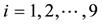
Example 3. Take into consideration the same two assets of Examples 1 and 2, with pay-off matrix,
 , and suppose that they are exchanged on the market as follows:
•
 has unit price 4 for (short) sales or purchases up to 10 units, 4.2 for purchases up to 50 units and 4.4 beyond 50 units;
•
 has unit price 5 up to 20 units, 5.5 up to 80 units and 6 beyond 80 units.
Such prices split the portfolio space into nine regions, identified by four vertices (see Figure 1).
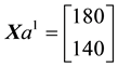
Let , and consider the portfolio
 . Of course,
 ; therefore,
 .Since
 is defined as the cheapest (super)hedge of W,
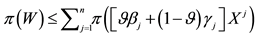 . On the other hand, the fact that all of the functions

 are convex w.r.t.
 implies that
 . By transitivity,
 , i.e. ,
 is convex.Note that this implies that the inequalities (3) hold for every
 , not just for the listed assets.•
 , which yields the pay-off
 and costs
 ;•
;• , which yields the pay-off
 and costs
 (recall thefirst 20 units of
 are bought at the cheaper price 5, and only the 60 subsequent units are bought at the higher price 5.5;•
 , which yields the pay-off
 and costs
 ;•
;• , which yields the pay-off
 and costs
 .Inside each region, the unit prices
 remain constant (shown in Figure 1 as well), and therefore the price functional
 is affine: we may write
 ,
, .In greater detail: there have to be nine vectors
 and nine (non positive) constants
Figure 1. The portfolio space in Example 3.
 such that, if
 with
with

 , then
 . Every vector

 identifies a discount factor
 and a risk-neutral probability
 , and therefore this model
identifies at least nine risk-neutral measures; however, as already pointed out, the risk-neutral measures turn out not to be as important as the properties of the price functional in order to investigate market efficiency.
Note that, if both X and
 belong to the same region
 , then
 : it is then straightforward to realise that, for every
 , the vector
 is easily determined by solving the usual linear system
 . The constants
 ,
,
 , are calculated as the amount “saved” by buying the “first” units at a price smaller than
 :
:
• In , the effective prices are the lowest ones: therefore,
 (we could argue the same conclusion from the fact that
 );
);
• In , the price of
 is 5.5, but the first 20 units are bought at the price
 , thus “saving”
 : therefore,
 (as a double check, consider for instance that the portfolio
 yields the pay-off
 and costs
 , and
, and
 pre-
pre-
cisely yields );
);
• In , the price of
 is 6, but the first 20 units are bought at
 less and the subsequent (
 ) 60 at
 less, for a total “saving” of
 : therefore,
 (note that such a saving can also be calculated as the one achieved in the “previous” region
 , i.e.,
 , plus the additional saving of 0.5 on all of the first 80 units:
 );
);
• In , the price of
 is 4.2, but the first 10 units are bought at
 less, thus “saving”
 : therefore,
 ;
;
• In , both the first 10 units of
 and the first 20 units of
 are bought at a lower price: the savings of
 and
and
 add up, and therefore
 ;
;
• In , the savings of
 and
and
 add up, and therefore
 ;
;
• In , the first 10 units of
 cost
cost
 less than the “full” price, and the subsequent (
 ) 40 cost
 less: the total saving is
 : therefore,
 ;
;
• In , the savings of
 and
and
 add up, and therefore
 ;
;
• Finally, .
.
Now, the price of every pay-off
 can be calculated as
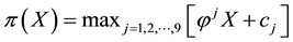 . For instance, for
 we get:
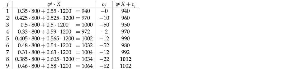
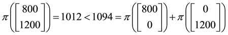
(the maximum price is emphasised). Note that, indeed, X is yielded by the portfolio , and the price of a is
 .
.
As already mentioned, the price functional
 is convex. We want nevertheless to strike out that, generally
speaking, it is neither sub- nor superadditive: for instance, consider again the pay-off . It is possible to check that
 and
and , and therefore
 . On the other hand, it is also
 , and therefore
 . We want to point out that this second inequality
does not correspond to a convenient super-hedging: indeed, it is not possible to buy simultaneously two portfo-
lios yielding the claim
 because, when doubling the position, the unit prices of the traded assets increase.
It is still possible to show that, if
 does not take infinite values, the set
 is compact and
convex. Mathematically speaking, the set
 is the union of the sub differentials of
 at all points
 ; note that, if
 is sublinear, then
 .
.
In perfect analogy to what happens for sublinear functionals,
 is increasing if and only if every
 is positive. The natural technique of pricing any pay-off Z (either belonging to
 or not) by super-hedging, as seen in Section 1.3, can still be applied, even in the case when
 allows for convenient super-hedgings, and it can be shown that the cheapest super-hedging price
 is a convex functional if the “original”
 is. Furthermore, the set
 corresponding to the set
 identified by
 turns out to be precisely the set
 .
.
Example 4. On
 consider the two assets:
• , at the unit price of 4.5, which increases at 4.7 for purchases of more than 10 units;
• , traded at 3.4 per unit, which increases at 3.7 for purchases of more than 20 units.
This way, . The prices split the portfolio space into four regions
 , corresponding to the four “quadrants” identified by the portfolio
 (see Table 1); note that the portfolio
 yields the pay-off
 and costs
 . The vectors
 and the constants
 , calculated as in
Table 1. The four regions of the portfolio space in Example 4.
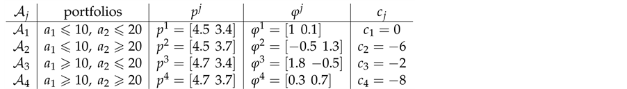
previous Example 3, are also shown.
There are positive vectors in
 (such as
 , for instance); yet, the negative components of
 and
and
 indicate the possibility of a convenient super-hedging. It is quite clear that such possibilities apply to all of the portfolios belonging to the regions
 and
and .
.
Consider, for instance, the portfolio , whose pay-off is
 and whose price is
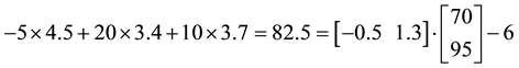 . It is immediate to check that the pay-off
 can be super-hedged by means of the portfolio
 , whose pay-off is
 and whose price is
 : a convenient super-hedging is found, and the cheapest super-hedging price functional
 will be such that
 (indeed, it can be shown that the equality holds).
Analogously, the portfolio
 yields the pay-off
 at the price
 , but a convenient super-hedging is given by
 , whose pay-off is
 and whose price is
 . Therefore,
 (and, as before, the equality holds, indeed).
It is possible to prove7 that the “adjusted” functional , calculated after exploiting all of the convenient super-hedgings, is calculated as the maximum of six affine functionals as shown in Table 2. Notably enough, the convex set
 identified by the six vectors
 exactly amounts to the subset of the positive vectors contained in the “original” set
 (see Figure 2). Note also that not all of the vectors
 ,
,
 , induce risk neutral measures, because some of them have negative components; however, each of the six “vertices” of the “restricted” set
 can again be seen as the product of a risk neutral measure and a discount factor (for instance,
 corresponds to the degenerate probability
 such that
 and to the discount fac-
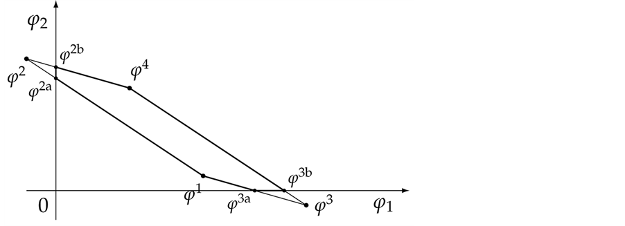
Figure 2. The sets
 (thin line) and
 (thick line) in Example 4.
Table 2. The four regions of the portfolio space in Example 4 after taking advantage of the convenient super-hedging opportunities.

tor ). Nevertheless, we remark that such elements are not as important as the js themselves to investigate market efficiency.
When it comes to positivity, things get a little more complicated: indeed, the fact that
 contains no positive functionals at all is still sufficient, but no longer necessary, in order to allow for arbitrages. Consider the following (and quite minimal) example.
Example 5. Again on , suppose that the asset
 is sold at the unit price 0.4 regardless of the amount, and that
 is sold at unit price
 up to 5 units, and 0.5 for more than 5 units. The portfolio space is trivially split into two regions (and in each of them, since
 , it is trivially
 ):
):

It is clear that arbitrages are possible, because buying
 with
with
 has a negative price for every
 . Nevertheless, the set
 contains the positive vector
 .
.
It is still possible to define the cheapest super-hedging price functional : it turns out that it simply amounts
to replace, in the region ,
,
 and
and
 with
with
 and
and . As a consequence, it is no longer
 : indeed,
 , which precisely indicates the possibility to get a free gain of 3 without risk. It is
also worth pointing out that such an arbitrage is just “local” in the spirit of Castagnoli et al. (2011) , in the sense that there is an upper bound to the gains that can be obtained by means of arbitrages.
The point is that, as already mentioned, an arbitrage is nothing but a convenient super-hedging of the null vector. In the sublinear case, positive homogeneity ensures that such a convenient super-hedging (meaning both its positive pay-off and its negative price) can be multiplied by an arbitrary positive constant and still remain an arbitrage: this way, if arbitrages are possible, the region of the arbitrage portfolios is always unbounded. In the “granular” convex case, instead, positive homogeneity no longer holds, and therefore arbitrages may be confined to a bounded region, as it happens in Example 5.
As a matter of fact, it is possible to show that a linear functional
 matters in determining whether
 allows for arbitrages or not only if
 is relative to a “region” of the portfolio space that contains the null pay-off: we call
 such a subset of
 8. In other terms, while
 is the union of all subdifferentials of
 , we are here only interested in the subdifferential
 of
of
 at the origin. Briefly, a convex functional
 is positive if and only if there exists a positive
 .
.
For sublinear functionals, it can be proven that the subdifferential at each point is by necessity a subset of the subdifferential at 0, or, in other words that . This, besides the “unbounded” nature of arbitrages in sublinear markets, provides a further argument in favour of the fact that, unlike what happens for convex markets, in sublinear markets absence of arbitrages and absence of convenient super-hedgings are properties of the same set L.
The results of this section can be summarized and formalized in the following
Theorem 1. Let
 be a linear space of financial assets, and
 be a convex pricing functional such that
 . Define
 and, for every
 , call
 and
and , so that
 . Let
. Let
 and
and . Then:
1. L is non-empty, closed and convex;
2. for every ,
, ;
;
3. for every ,
,
 and
and
 is linear; furthermore, there exists
 such that
 ;
;
4.
 and
and
 are non-empty, closed and convex, and
 ;
;
5.
 is increasing if and only if every
 is positive;
6.
 is positive if and only if there exists a positive
 .
.
3. Increasing Average Prices
The Star-Shaped Case
Suppose that
 is such that the supply and demand function
 is convex. If, as it is natural to suppose,
 , then it turns out that
 (3)
(3)
the first inequality comes from the convexity property, because (being ) it is
 ; it is furthermore possible to see that the two inequalities are equivalent to each other9.
A possible reason why inequalities (3) are sensible in ordinary markets can be seen as follows. Take
 such that
 , so that
 . The first of the two inequalities (3) above is equivalent to

in other words, the supply and demand function of an
 satisfies (3) if and only if the average unit price of X is increasing with respect to the traded amount. This is why we deem reasonable such a property: indeed, when aiming at purchasing some quantity of something, it is rational to buy it at the lowest possible overall price, which of course coincides with the lowest average unit price.
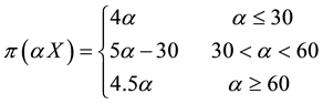
Suppose, for instance, that three agents sell the same asset X on the market. The first one sells it at 4 per unit, but can only provide up to 30 units. The second one sells it at 5 per unit (for any amount). The third one sells it at 4.5 per unit, but only for a minimum order of 50 units. It is clear that the best price that can be obtained to buy
 units of X are:
for instance, to buy 50 units of X, the unit price of 4.5 may be obtained, but it is less expensive to buy 30 units from the first agent and 20 from the second, at a total price of
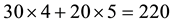 instead of
 . Note that the average price obtained with the “separate” purchase is
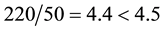 .
.
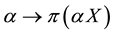
We shall call star-shaped a supply and demand function
 that satisfies inequalities (3) and, in general, any function
 , with
 any real linear space, that does the same. Note the difference with “granular” pricing functionals, which feature an increasing marginal price with respect to the traded amount: of course every convex function is star-shaped as well, but the converse need not be true.
Example 6. The function
 defined as
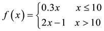
is star shaped, because ( and) its “average value”
 is increasing. Nevertheless, f is not convex (and not even continuous).
A geometrical interpretation of the star-shaped property is easily deduced from the monotonicity of average prices. Recall that, given any real linear space , a function
 is convex if and only if, whenever two points
 are given “above” the “graph” of f, i.e., such that

 , then the entire segment adjoining
 and
and
 remains “above” the graph of f (which translates into
 for every
 ). The property that average prices are increasing for star-shaped functions translates into the fact that whenever
 is given “above” the “graph” of f, i.e., such that
 , then the entire segment adjoining
 and
and
 remains “above” the graph of f (which translates into
 for every
 ). In Figure 3 the typical appearance of the four functions examined in this paper is depicted for functions
 .
.
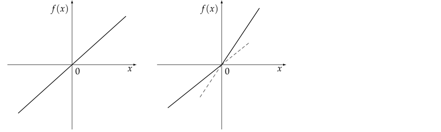 (a) (b)
 (c) (d)
Figure 3. Typical graphs of (a) a linear function; (b) a sublinear (and not linear) function; (c) a convex (and not sublinear) function and (d) a star-shaped (and neither convex nor continuous) function.
Suppose that, in an exchange list under consideration, the assets
 are included, such that, for every
 , the supply and demand function
 is increasing and star-shaped. Once again, we define on the set
 of all attainable pay-offs a price functional
 by super-hedging:

As usual, such a functional immediately turns out to be increasing (and therefore positive, because ); moreover, it can be proved that
 is star shaped as well, i.e., that inequalities (3) hold for every
 . So to say, the star-shape of the single supply and demand functions “propagates” by super-hedging.
An adaptation of a result by
Chateauneuf & Aouani (2008)
, still unpublished (see
Castagnoli et al., 2009
), shows that a star-shaped functional
 can be represented as the pointwise minimum of the convex functions that dominate it. In detail:
Proposition 2. Let
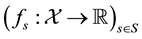
 be a star-shaped functional. Then the set
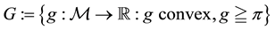 is closed and convex, and
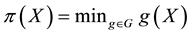 for every
 .
.
It is indeed possible to prove that only the convex functionals
 such that
 can be taken into consideration, i.e., that if
 , then (
 is closed and convex as well and)
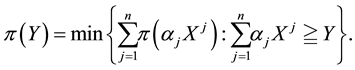
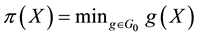 as well. By applying Proposition 1, we can write each
 as in (2), and therefore represent the star-shaped functional
 as
as
 (4)
(4)
To give an economical interpretation of such a representation, think that several agents are available to sell X on the market. Each agent, corresponding to a , assigns a convex price to X (i.e., has an increasing marginal price), and we are free to choose the agent we want to buy the asset X from (i.e., the cheapest one).
It is worth mentioning that the class of star-shaped functionals is closed under pointwise sup and inf, even for an infinite family of functionals; more explicitly, if
 is any real linear space and
 is a family of star-shaped functionals such that
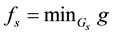 , then
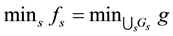 and
and .
.
Example 7. Take into consideration the same two assets of Examples 1, 2, and 3, with pay-off matrix
 We suppose that the investor can call her/his demands on three different markets, each run by a (representative) agent with her/his own convex price system: this way, three convex price functionals
 ,
,
 and
and
 are given. Suppose that the first one is the same of Example 2, with nine portfolio region as follows:

The second agents gives the granular price functional
 identified by10
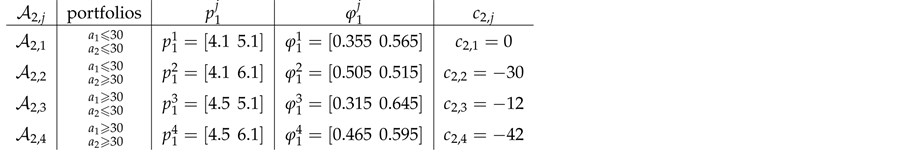
The third agent simply gives a linear price: ,
, .
.
Let us take into consideration some random variables: the details of the calculations (which amount to see in which region the price of the given pay-offs is maximum) are left to the reader.
• For , it is
 ,
,
 , and
, and : therefore,
 is bought from the second agent and
 .
.
• For , it is
 ,
,
 , and
, and : therefore,
 is bought from the first agent and
 .
.
• For , it is
 ,
,
 and
and : therefore,
 is bought from the third agent and
 .
.
It is then clear that each of the three price systems has a chance to prove the cheapest one and, therefore, that it is effective in determining
 as the pointwise minimum of
 ,
,
 , and
, and . This can happen even for a
single asset: for instance, the three demand functions
 for
for
 in the three mar-
kets turn out to be:
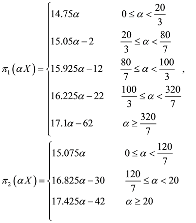
and . It is straightforward (but very laboured) to see that
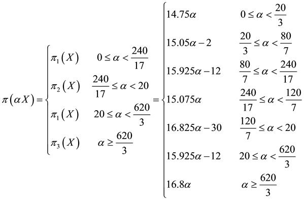
note that the marginal price is not increasing (for instance, around , it decreases from 15.925 to
15.075), whereas the average one is.
It is still true that the star-shaped price functional
 does not allow for convenient super-hedgings if and only if it is increasing.
Notably, if this is the case, instead of the set
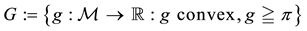 of Proposition 2 or the set
 of (4), the subsets
 and
and
 can be taken into consideration in order to represent
 . Define indeed, for every
 , the functional
 by
by : the fact that g is convex ensures that such a minimum exists. It is clear that
 is increasing and that
 ; furthermore, it is possible to prove (by taking into consideration the monotonicity of
 ) that still
 .11 This way, it is straightforward to realise that
 and, therefore, that
 for every
 .
.
Since it is trivial that the minimum of a family of increasing functionals remains increasing, the above considerations allow us to conclude that a star-shaped functional does not allow for convenient super-hedgings if, and only if, it can be represented as the pointwise minimum of a family of increasing functionals. Note that this is quite analogous to what happened for convex and, before, for sublinear functionals:
 allows for no convenient super-hedgings if, and only if, all of the functionals in the representation of
 are increasing.
In order to deal with arbitrages, one more consideration is needed. Since, in the economical interpretation we gave, we are free to choose, among several agents, the best one to buy the pay-off X we want to detain, it is reasonable to think that we may prefer to buy several different portfolios from the different agents, in such a way that the overall position matches or, better, super-hedges X. Mathematically speaking, we are dealing with the following object:
Definition 1. Let
 be a real linear space, and
 a family of real functionals on
 . The inf-convolution of G is the functional
 defined by, for every
 ,
,
This way, if we are given a set
 of price functionals, each ideally corresponding to a different market (or agent), taking their inf-convolution amounts to buying a finite number of positions
 , on the markets
 respectively, in such a way that the overall pay-off
 super-hedges the desired pay-off X. Note that, as a consequence, the inf-convolution of a family of functionals always turns out to be smaller than their pointwise minimum. (Note also that, if the
 are all increasing, the condition
 can be equivalently replaced by
 .)
.)
The following proposition holds true, with evident consequences from the financial point of view.
Proposition 3. Let
 be a real linear space and
 be a family of real functionals on
 such that every
 is increasing and such that
 . Let
. Let
 be the inf- convolution of G: then F is finite-valued, and
1. if every
 is convex, then F is convex;
2. if every
 is star-shaped, then F is star-shaped.
The fact is that, even if every
 is such that
 , it is not necessary that
 . Economically speaking, even if the “original” markets do not allow either for arbitrages nor for convenient super- hedgings, a “cross-market” arbitrage may still be possible.
Example 8. Consider again the three markets of Example 7: we saw that
 can be bought from the second agent at the price 276. It is immediate to check that for
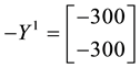 it is
it is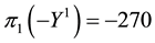 ,
,
 , and
, and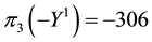 : therefore,
 can be sold to the third agent for a gain of 306, thus making a “cross-market” arbitrage of 30.
As a consequence, the inf-convolution
 of
of
 will be star-shaped and increasing, because of
Proposition 3, but such that . (The inequality is indeed strict: for instance,
 , and
, and ).
).
Although the technical details for a complete proof become too complex to be reported here, the key feature can be guessed from the following (and last) example.
Example 9. The function

is increasing, star-shaped and such that . Yet, it is clear that
 and
and , so that
 . Note that the subdifferential of f at 0 is the empty set (no straight line fits below the graph of f).
The point that can be proven is that, if a star-shaped price functional is the result of a “best price” over several markets, “cross-market” arbitrages are possible if and only if there are assets whose price around 0 behaves like the function of Example 9. Therefore, the same condition seen for convex functionals applies: a star-shaped price functional does not allow for arbitrages, not even cross-market ones, if and only if the subdifferential
 of
of
 at 0 contains at least a positive functional
 . If
. If , of course such a condition is not satisfied, which immediately signals the possibility of arbitrages.
Note that cross-market convenient super-hedgings may still be possible, as Example 8 itself makes clear12: as a consequence of Proposition 3, this is of course bound to happen every time that the price function is (star- shaped but) not convex.
We can summarise the results of this section in the following:
Theorem 2. Let
 be a linear space of financial assets, and
 be a star-shaped pricing functional such that
 . Define
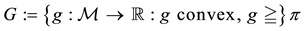 and
and . Call
 and
and . Finally, call F the inf-convolution of G (see Definition 1) and define, as in Theorem 1,
 . Then:
1. G and
 are non-empty, closed and convex;
2. for every ,
, ;
;
3.
 is increasing if and only if
 for every
 .
.
4.
 is positive if and only if there exists a positive
 .
.
Remark 3. In this section, we have seen two ways to build the overall supply and demand function of a given asset in the case when several “markets” are available.
1. In the first case, seen at the beginning of the section, we supposed that the agent simply chooses the “best market”: implicitly, we imposed that every single trade can only happen with a single agent. In such a case, the market is chosen where the total price, or (which is the same) the average price, is the minimum one.
2. In the second case, by using the “inf-convolution” technique, we supposed that the agent is free to split the desired position into “chunks” and buy the various “chunks” separately on the various markets. This way, for every single additional unit, the agent chooses the market where the marginal price is the minimum one.
Depending on the type of price functionals on the “original” market, we saw that:
1. In the first case, when all of the markets feature either a convex or a star-shaped price functional, the overall price functional turns out to be star-shaped: we pointed indeed out that an increasing average price is obtained;
2. In the second case, the overall price functionals inherit the convexity or the star-shape of the original functions (namely, it is convex if all of the original pricing functionals are, and star-shaped likewise): the minimum marginal price is chosen, and yet it need not be increasing unless it is in the original markets already.
In some sense, we have found that convexity and star-shape are quite “stable” properties in financial markets.
Of course, several other “rules” can be imagined: for instance, some markets may be only available for purchases, or for sales, or only some particular amounts can be bought (not just with a minimum or a maximum amount, as seen in the beginning of this section, but for instance for multiples of some “size” only), in such a way that the offer price function turns out not even to be star-shaped. Anyway, examining such cases goes beyond the scopes of the present paper.
4. Analysis
Four type of price systems, each a generalisation of the previous one, have been examined in this paper. From the last to the first, they are:
1. star-shaped prices:

2. convex (or granular) prices, obtained when G is a singleton:
3. sublinear prices, obtained when (G is a singleton and)
 (and therefore
 ) for every
 :
:
4. linear prices, obtained when (G is a singleton,
 for every
 , and furthermore) L is a singleton:
The mentioned fact that both the pointwise minimum and the inf-convolution of a family of star-shaped functionals still are star-shaped seems to suggest that no further generalisation of this type should be fruitful.
For each of the above types, the conditions for absence of arbitrages and of convenient super-hedgings can be examined by taking into consideration the behaviour of the price functionals on the indicator functions
 with
with
 (where, as usual,
 if
if
 and =0 otherwise), which are all positive.
1. Linear prices: . The price of
 is the value
 : it is then immediate that such a price is positive for every A (i.e., that no arbitrages and no convenient super-hedgings are possible) if and only if
 . Intuitively, indeed, if
 is not positive, then there exists an
 13 such that
 , so that
 makes an arbitrage.
2. Sublinear prices: , with
 . Recall that the positivity of
 is equivalent to the positivity of its ask prices, and its (increasing) monotonicity is equivalent to the positivity of its bid prices. The ask price of
 is
is
 and its bid price is
 : therefore, the ask price is positive as soon as one of the prices
 is, i.e., if there exists a positive
 , and the bid price is positive only if all of the prices
 are, i.e., if all
 are positive. Intuitively, if there is a non-positive
 , then as above there exists an
 such that
 : this means that
 , so that
 makes a convenient super-hedging of the null pay-off. Less intuitively, and indeed harder to prove, if all
 are not positive, then there exists an
 such that
 for every
 : in this case,
 , and
, and
 makes an arbitrage.
3. Convex prices: , with
 . Call
 the set of all
 such that
 for some
 . The ask price of
 is positive as soon as
 is: since
 , this implies that
 is increasing, i.e., positive, that is to say, that there exists a positive
 in
in .
.
As for arbitrages, since
 is not positively homogeneous, we need to take into consideration every
 for
for : in order to make an arbitrage,
 has to be negative for all
 and for some
 . This happens if
 for every
 : since this equality can be easily met when
 (it is
enough to take
 “small enough”), indeed only the
 such that
 can be taken into consideration, and these fs (which amount to the set
 of the linear functionals of L) are precisely the ones that concur in determining the value of
 close to 0. Therefore, the above arguments for sublinear functionals can be repeated in a “local” sense (i.e., for a
 with
with
 “small enough”), to conclude that
 does not allow for arbitrages if there exists a positive
 .
.
Intuitively, if there is a non-positive , then as above there exists an
 such that
 : since there is some
 such that
 , it is possible to get also
 if k is “big enough”, and this means that
 (convenient super-hedging). On the other hand, if all
 are not positive, then there exists an
 such that
 for every
 : in this case, it is possible to choose k “small enough” so as to obtain
 , and
, and
 makes an arbitrage.
4. Star-shaped prices: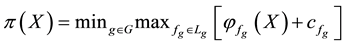 . The ask price of
 is positive only if all of the
 are positive for every convex
 : in other words,
 does not allow for arbitrages only if
all
 do not allow for them. As for convenient super-hedgings, it is now quite complex to summarise the properties that have to be imposed on the convex functionals
 in order to get an increasing functional
(for instance, it is possible to prove that, for every ,
, : an increasing
functional, i.e., the identity , is obtained as the pointwise minimum of a family of functions, none of which is increasing). We have nevertheless realized that, if
 is increasing, then only the increasing functionals
 may be taken into consideration and, on the other hand, that the pointwise minimum of increasing functions is increasing: therefore,
 does not allow for arbitrages if it can be written as the minimum of a family of increasing convex functionals14. Intuitively, it is clear that an arbitrage is possible as soon as even a single market allows for it, but now, for convenient super-hedgings, things become quite different. Indeed, recall that a convenient super-hedging is a pair
 such that
 but
but : in order to “deactivate” such a situation, i.e., in order to obtain
 , it may be enough that on a single market Y is sold at a cheaper price than
 .
.
It is clear that moving from linear to star-shaped price systems yields price systems whose properties are closer and closer to what happens in “real” financial markets. Yet, because of the fact that such systems are each the generalisation of the previous one, the “efficiency” conditions for each family of functionals propagates on the further generalisations in a reasonable way. All in all, therefore, these four price systems altogether make quite a versatile toolbox for building financial models, in the sense that, when a financial model is needed, it is easy to “fine tune” the level of precision to suit the needs of the considered problem.
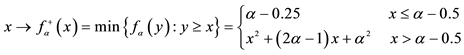
which are all convex and increasing.
5. Conclusion
A classical problem in Mathematical Finance is to study the prices of a suitable set of risky financial assets, modeled as random variables on some state sets, by means of suitable functionals defined on this set of random variables. The properties of the price functional reflect the assumptions on the market. In this paper, we analysed four types of price functionals. We first summarized the properties of the widely known linear functionals, obtained when the market was supposed to be perfect, and of sublinear functionals, which took into account the proportional frictions. Then, we introduced two more classes of functionals which accommodate a wider set of market frictions: granular (convex) functionals, obtained when the unit prices of traded assets were increasing w.r.t. the traded amount, and star-shaped functionals, obtained when the average unit prices of traded assets were increasing w.r.t. the traded amount. We explored some characterizations of such functionals, together with their relationships with arbitrages and market inefficiencies, and performed a final analysis on their effectiveness in allowing for versatile modelling.
Cite this paper
ErioCastagnoli,Marzia DeDonno,GinoFavero,PaolaModesti, (2015) Granular and Star-Shaped Price Systems. Journal of Financial Risk Management,04,227-249. doi: 10.4236/jfrm.2015.43018
References
- 1. Artzner, P., Delbaen, F., Eber, J. M., & Heath, D. (1999). Coherent Measures of Risk. Mathematical Finance, 9, 203-228.
http://dx.doi.org/10.1111/1467-9965.00068 - 2. Björk, T. (1999). Arbitrage Theory in Continuous Time. Oxford: Oxford University Press.
- 3. Black, F., & Scholes, M. (1973). The Pricing of Options and Corporate Liabilities. Journal of Political Economy, 81, 637-654.
http://dx.doi.org/10.1086/260062 - 4. Castagnoli, E., Favero, G., & Maccheroni, F. (2009). Marchetto, il prezzatore perfetto. Elogio dell'internalità. Milan: Electronic Draft.
- 5. Castagnoli, E., Favero, G., & Modesti, P. (in print). Price Systems for Random Amounts: A Unified Approach. In D. Jakóbczak (Ed.), Analyzing Risk through Probabilistic Modeling in Operations Research. Hershey: IGI Global.
- 6. Castagnoli, E., Favero, G., & Tebaldi, C. (2011). One-Penny Arbitrages, or: A Free Snack without a Free Lunch. Journal of Applied Computer Science & Mathematics, 10, 20-21.
- 7. Cerreia-Vioglio, S., Maccheroni, F., Marinacci, M., & Montrucchio, F. (2011). Risk Measures: Rationality and Diversification. Mathematical Finance, 21, 743-774.
- 8. Chateauneuf, A., & Aouani, Z. (2008). Exact Capacities and Star-Shaped Distorted Probabilities. Mathematical Social Sciences, 56, 185-194.
http://dx.doi.org/10.1016/j.mathsocsci.2008.01.006 - 9. Cvitanic, J., Pham, H., & Touzi, N. (1999). A Closed-Form Solution for the Problem of Super-Replication under Transaction Costs. Finance and Stochastic, 3, 35-54.
http://dx.doi.org/10.1007/s007800050051 - 10. Davis, M. H. A., & Clark, J. M. C. (1994). A Note on Super-Replicating Strategies. Philosophical Transactions: Physical Sciences and Engineering, 347, 485-494.
- 11. de Finetti, B., & Obry, S. (1933). L’optimum nella misura del riscatto. Atti del Secondo Congresso Nazionale di Scienza delle Assicurazioni, 2, 99-123.
- 12. Delbaen, F., & Schachermayer, W. (1994). A General Version of the Fundamental Theorem of Asset Pricing. Mathematische Annalen, 300, 463-520.
http://dx.doi.org/10.1007/BF01450498 - 13. Dothan, M. U. (1990). Prices in Financial Markets. Oxford: Oxford University Press.
- 14. El Karoui, N., & Quenez, M. C. (1995). Dynamic Programming and Pricing of Contingent Claims in an Incomplete Market. SIAM Journal on Control and Optimization, 33, 29-66.
http://dx.doi.org/10.1137/S0363012992232579 - 15. El Karoui, N., & Ravanelli, C. (2009). Cash Sub-Additive Risk Measures and Interest Rate Ambiguity. Mathematical Finance, 19, 561-590.
http://dx.doi.org/10.1111/j.1467-9965.2009.00380.x - 16. Föllmer, H., & Schied, A. (2002). Convex Measures of Risk and Trading Constraints. Finance and Stochastic, 6, 429-447.
http://dx.doi.org/10.1007/s007800200072 - 17. Hodges, S. D., & Neuberger, A. (1989). Optimal Replication of Contingent Claims under Transaction Costs. The Review of Futures Markets, 8, 222-239.
- 18. Jouini, E. (1997). Market Imperfections, Equilibrium and Arbitrage. Lecture Notes in Mathematics, 1656, 247-307.
http://dx.doi.org/10.1007/BFb0092002 - 19. Jouini, E., & Kallal, H. (1995). Martingales and Arbitrage in Securities Markets with Transaction Costs. Journal of Economic Theory, 66, 178-197.
http://dx.doi.org/10.1006/jeth.1995.1037 - 20. Koehl, P. F., & Pham, H. (2000). Sublinear Price Functionals under Portfolio Constraints. Journal of Mathematical Economics, 33, 393-399.
http://dx.doi.org/10.1016/S0304-4068(99)00024-5 - 21. Merton, R. (1973). Theory of Rational Option Pricing. Bell Journal of Economics and Management Science, 4, 141-183.
http://dx.doi.org/10.2307/3003143 - 22. Pham, H., & Touzi, N. (1999). The Fundamental Theorem of Asset Pricing with Cone Constraints. Annals of Mathematical Economics, 31, 265-279.
http://dx.doi.org/10.1016/s0304-4068(97)00059-1 - 23. Pliska, S. (1997). Introduction to Mathematical Finance: Discrete Time Models (2nd ed.). Malden: Blackwell.
- 24. Rockafellar, R. T. (1970). Convex Analysis. Princeton: Princeton University Press.
http://dx.doi.org/10.1515/9781400873173 - 25. Stewart, I., & Tall, D. (1983). Complex Analysis. Cambridge: Cambridge University Press.
NOTES

*Corresponding author.

1Further generalisations of convex risk measures have been proposed. El Karoui & Ravanelli (2009) remarked that cash additivity, which was a required property of coherent risk measures, should be replaced with cash subadditivity in several cases (e.g., with lack of liquidity for the “riskless” asset). Starting from this, Cerreia-Vioglio et al. (2011) proposed to replace convexity with quasi-convexity in order to better maintain the financial meaning of “diversification” originally connected with the subadditivity requirement. An interpretation of such generalisation in terms of financial prices, though, does not appear to be immediate, and is still under investigation.

2A puzzled reader, wondering about the measurability of such random variables, will find some clarifications in Remark 1 below.

3It is natural to wonder whether such a j always exists. It can be shown (see Pliska, 1997 and Castagnoli et al., 2009 ) that existence is guaranteed by a weaker condition than the absence of arbitrages, called the law of one price (roughly speaking, there is no way to obtain the same pay-off at two different prices): this always happens if, as in this example, the pay-off of the listed assets are linearly independent.

4The dual of the problem
 is
is , which can be written as
 ; the dual of
 is
is .
.
5Suppose that
 are such that
 . This means that every portfolio that super-hedges Y super-hedges Z: therefore, the min that corresponds to the super-hedging price
 is evaluated on a subset of the set where the min corresponding to
 is evaluated. As a consequence,
 .
.

6To prove the inequality, suppose that the cheapest (super) hedges for
 are, respectively,
 and
and , so that
 and
and .
.

7We confine ourselves to a few hints, in order to help a reader possibly interested in finding a method into this madness. In the region , the “marginal” pay-off
 (yielded by the “marginal” portfolio
 ) has a negative cost (indeed,
 ): therefore, the idea is to add to any portfolio
 a multiple of
 until “hitting” the boundary with another region. If
 , such a region turns out to be
 , and the affine pricing functional used to price the pay-off becomes
 ; in the opposite case when
 , the region hit is
 , and the “adjusted” pricing functional is
 . Analogous considerations apply to the region
 , where the “marginal arbitrage” is the pay-off
 , (yielded by the marginal portfolio
 ), which costs
 .
.

8In the case when ,
,
 can also be defined as the subset of linear (not just affine) functionals of
 or, equivalently, as the set of all
 such that
 .
.

9Define, indeed
 and
and : it is clear that
 (respectively,
 ) if and only if
 (respectively,
 ) and that
 can be written as
 , i.e. ,
 .
.

10We are supposing here that the three “markets” share the exchange list, i.e., that the same assets are exchanged on the three markets. This is just chosen in order to avoid further complications: indeed, on different markets, different assets could be quoted and exchanged.

11For every , it is
 for some
 ,
, . It is
 because
 ; therefore, by monotonicity of
 , we get that
 .
.

12In Example 8, buying
 on the first market and
 on the second one costs less than buying
 on the cheapest ( i.e., still the second) one.

13In the spirit of Remark 1, we should write .
.

14To conclude the short example: in computing , for every
 , instead of the functions
 it is possible to take into consideration the functions