American Journal of Climate Change
Vol.05 No.02(2016), Article ID:67721,16 pages
10.4236/ajcc.2016.52021
Case Study: A Simulation Model of the Spawning Stock Biomass of Pacific Bluefin Tuna and Evaluation of Fisheries Regulations
Kazumi Sakuramoto
Department of Ocean Science and Technology, Tokyo University of Marine Science and Technology, Tokyo, Japan

Copyright © 2016 by author and Scientific Research Publishing Inc.
This work is licensed under the Creative Commons Attribution International License (CC BY).
http://creativecommons.org/licenses/by/4.0/


Received 1 April 2016; accepted 21 June 2016; published 26 June 2016
ABSTRACT
This study proposes a simulation model that well reproduces the spawning stock biomass of Pacific bluefin tuna. Environmental factors were chosen to estimate the recruitment per spawning stock biomass, and a simulation model that well reproduced the spawning stock biomass was developed. Then, effects of various fisheries regulations were evaluated using the simulation study. The results were as follows: 1) arctic oscillations, Pacific decadal oscillations and the recruitment number of the Pacific stock of Japanese sardine were chosen as the environmental factors that determined the recruitment per spawning stock biomass; 2) spawning stock biomass could be well reproduced using a model that reproduced the recruitment per spawning stock biomass and the survival process of the population that included the effect of fishing; and 3) the effects of various fisheries regulation could be evaluated using the simulation model mentioned above. The effective regulation in the simulations conducted in this paper was a prohibition of fishing for 0- and 1-year-old fish in terms of recovering the spawning stock biomass. The reduction of fishing mortality coefficients for all age fish to 50% of actual values also showed a good performance. The recent reductions of the recruitment and spawning stock biomass were likely caused by heavy harvesting, especially of immature fish, since 2004.
Keywords:
Bluefin Tuna, Recruitment, Spawning Stock Biomass, Stock-Recruitment Relationship, Fisheries Regulation, Arctic Oscillation (AO), Pacific Decadal Oscillation (PDO)

1. Introduction
The abundance of Pacific bluefin tuna, Thunnus thynnus, has seriously decreased in recent years. In 1952, the starting year of the current stock assessment, total stock biomass was 119,400 t. During the stock assessment period, the total stock biomass reached the historical maximum of 185,559 t in 1959, and a historical minimum of 40,263 t in 1983. Total stock biomass started to increase again in the mid-1980s and reached its second highest peak of 123,286 t in 1995. Total stock biomass decreased throughout 2008-2012, averaging 50,243 t per year, but reached 44,848 t in 2012 [1] . Recovering the stock abundance has become an urgent issue. In order to discuss optimal management procedures, it is important to understand the Stock-Recruitment Relationship (SRR) for this species; however, a clear relationship between Recruitment (R) and Spawning Stock Biomass (SSB) has not been detected, and the recruitment seems to fluctuate regardless of the level of SSB. Whether or not a clear relationship between R and SSB can be detected is important, because if R does not show a clear relationship to SSB, we cannot expect a fisheries regulation directly aimed at increasing R to have any effect on the end-goal, which is to increase SSB. In this case, the more effective regulation would be to manage the population after they are recruited.
Recently, however, Sakuramoto [2] - [4] proposed a new SRR model that incorporated environmental factors instead of assuming a density-dependent effect. That is,
 (1)
(1)
where Rt and St-1 denote the recruitment in year t and spawning stock biomass in year t-1, respectively. The f(.) denotes a function that evaluates the effects of environmental factors in year t. The variable  is a vector representing the environmental factors, comprised not only of physical factors such as water temperatures, but also biological interactions such as a prey-predator relationship. The parameter k denotes the number of environmental factors. That is, Rt is proportionally determined by St-1, and simultaneously, Rt is affected by environmental factors in year t. In this study, the Arctic Oscillation (AO) by month and Pacific decadal oscillation (PDO) by month were examined as the environmental factors. As the factors of biological interactions, we examined the R and SSB of the Pacific stock of Japanese sardine, which was one of the main prey populations for Pacific bluefin tuna.
The purpose of this study is to investigate whether or not the SRR model described by equation (1) is applicable to Pacific bluefin tuna, and can reproduce the trajectory of SSB. Another aim of this study is to evaluate the effect on SSB of fisheries regulations for Pacific bluefin tuna using the simulation model developed in this study.
2. Methods
2.1. Data
The data used in this study are as follows: 1) Recruitment of Pacific bluefin tuna, derived from the report of the International Scientific Committee (ISC) [1] , and the Pacific stock of Japanese sardine [5] [6] , defined by the number of 0-year-old fish in year t, from 1953 to 2012; 2) the SSB of Pacific bluefin tuna from 1952 to 2012 [1] and the Pacific stock of Japanese sardine [5] [6] from 1953 to 2012; 3) the fishing mortality coefficient at age a in year t for Pacific bluefin tuna from 1953 to 2012 [1] ; 4) Arctic Oscillation (AO) by month from 1953 to 2012 [7] ; 5) Pacific decadal oscillation (PDO) by month from 1953 to 2012 [8] ; 6) maturity rate values of 0 for 0-, 1- and 2-year-old fish, 0.20 for 3-year-old fish, 0.50 for 4-year-old fish, and 1.0 for 5-year-old and older fish [1] ; 7) the natural mortality coefficients for 0-, 1-, and 2+-year-old fish of 1.36, 0.76 and 0.25, respectively [1] ; and 8) mean weight by age taken from the ISC [1] , with the mean weight of age all fish age 10 and older combined as a single value, as determined by the following equation:
 (2)
(2)
where 0.25 is the natural mortality coefficient for ≥10-year-old fish. Otherwise, the average weights by age were calculated using the growth curve and length-weight relationship used in the ISC [1] .
All the data used in this study can be easily obtained through the internet. However, Sakuramoto [2] pointed out that the fishing mortality coefficients for the Pacific stock of Japanese sardine since 2001 were overestimated, and that the previously estimated values were acceptable if halved. Therefore, according to Sakuramoto [2] , the recruitment for year 2001 to 2012 should be modified as follows:
 (3)
(3)
where M is 0.4, which is the natural mortality coefficient for the Pacific stock of Japanese sardine for age 0, and Ft,0 denotes the fishing mortality coefficient for the Pacific stock of Japanese sardine for age 0 in year t. The average of dift was 1.826, which corresponded to 6% - 9% of the observed ; then ln (1.826) was added to the
  after 2001. The modified
  values are shown in Table 1.
2.2. Estimation of the Model that Reproduces RPS
As the environmental conditions, AO in month m of year t,  , (m = Jan., Feb,…, Dec.), and PDO in month m of year t
 , (m = Jan., Feb,…,Dec.) were examined. As factors of biological interactions, the R and SSB of the Pacific stock of Japanese sardine were examined. Parameter selection was done by a stepwise method using the free software R version 2.12.1.
2.3. Construction of a Model that Reproduces SSB
The procedure to reproduce SSB is shown in Figure 1.
Step 1: The initial values of population at age a in year 1953,  (0 ≤ a ≤ 10+), are given, based on the ISC [1] .
Step 2: SSB in year t,  , (1953 ≤ t ≤ 2012) is calculated using the following equation:
 (4)
(4)
where ma and wa denote the maturity rate and mean weight at age a.

Table 1. Number of recruitment for the Pacific stock of Japanese sardine, from 1953 to 1975 was referred to Yatsu et al. [5] , from 1976 to 2012, was referred to Kawabata et al. [6] , from 2001 to 2012 was modified, in this study, which are shown with asterisks.
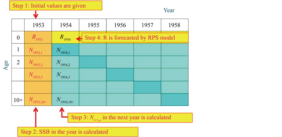
Figure 1. The procedure of the simulation that reproduces R and SSB.
Step 3: The number of individuals at age a in the next year t + 1 (1 ≤ a ≤ 10+, 1953 ≤ t ≤ 2011),  , is calculated using the following equation (Here,
  denotes the number of individuals at age 10 and older in year t + 1):
 (5)
(5)
 (6)
(6)
Step 4: Recruitment in the next year t + 1 (1953 ≤ t ≤ 2011) is calculated using the following equation:
 (7)
(7)
Here,  is calculated using the model determined in the previous section.
Step 5: Catch at age a (0 ≤ a ≤ 10+) in year t + 1 (1952 ≤ t ≤ 2011) is calculated using the following equation:
 (8)
(8)
2.4. Evaluation of the Fisheries Regulations
The effects of fisheries regulations were evaluated using simulation studies. As we show the trajectory of SSB later, the SSB was very low in the middle of 1980s. Then we assumed that a regulation was commenced for 5 years from 1987 to 1991 (Table 2). The other years and duration can be assumed a priori.
Scenario A1 is the case when all the fishing mortality coefficients for age 0 to (10+)-year-old fish were reduced to 50% of the actual values. Scenario A2 is the case in which fishing for age 0- and 1-year-old fish was prohibited. That is, the fishing mortality coefficients for 0- and 1-year-old fish were set at zero in the simulation. Scenario A3 is the case when fishing mortality coefficients for 0- to 3-year-old fish were reduced to 50% of the actual values. Scenario A4 is the case when fishing the only prohibition was against catching fish less than 1 year old.
The effect of the regulation for SSB in year t, ESt, is evaluated using the following equations:
 (9)
(9)
Table 2. Fisheries regulations commenced for 5-year from 1987 to 1991 (A1-A4), and those commenced for 9-year from 2004 to 2012 (B1-B4). Fa, ISC denotes the fishing mortality coefficient derived from the ISC [1] .
 (10)
(10)
Here,  denote the R and SSB in year t reproduced by the simulation in which no fisheries regulation was introduced, and
  denote the resultant R and SSB in year t when a fisheries regulation was introduced.
The effect of the regulation for catch in year t, ECt, is evaluated using the following equations:
 (11)
(11)
Here,  denotes the catch at age a in year t calculated when the fisheries regulation was introduced, and
  denotes the catch at age a in year t reproduced by the simulation in which no fisheries regulations were introduced.
2.5. Cause of the Recent Reduction of R and SSB
In order to evaluate the cause of the recent reduction of R and SSB, simulations were conducted on the fisheries regulations that commenced from 2004 to 2012 (Table 2), because the catch has greatly increased since 2004 and the SSB has continued to decrease as shown in the results section. Scenario B1 is the case when the fishing mortality coefficients for all fish were reduced to 50% of the actual ones. Scenario B2 is the case when the fishing for 0- and 1-year-old fish was prohibited. Scenario B3 is the case in which the fishing mortality coefficients for 0- to 3-year-old fish were reduced to 50% of the actual values, and scenario B4 is the case when the fishing for 0-year-old fish was prohibited.
3. Results
3.1. Estimation of the Model that Reproduces RPS
The following model was selected by the stepwise method, which made the AIC being the minimum (AIC = −68.00)
 (12)
(12)
where the figures in the suffixes for A and P denote the month in AO and PDO, respectively. The RSardine, t denotes the recruitment of the Pacific stock of Japanese sardine in year t. The RPS reproduced by this model, which was transformed from ln (RPS), is shown in Figure 2. The observed RPS, which refers to the ISC [1] , was extremely high in 1990, and could not be reproduced by this model. The observed RPS values were higher than those reproduced in 1973, 2004 and 2008, and the opposite cases occurred in years 1955, 1956, and 1982.
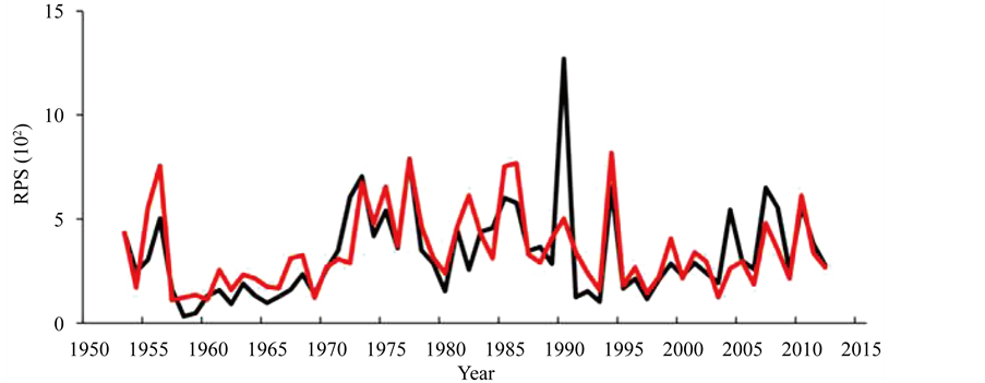
Figure 2. RPS produced by simulation model (red) and based on ISC data [1] (black).
However, for the other years, the reproduced and observed RPSs coincided well.
3.2. Sensitivity Tests for Models to Reproduces RPS and R, Respectively
We conducted sensitivity tests on models intended to reproduces ln (RPS) and ln (R), respectively. Table 3 shows the dependent variables, factors that were used as the candidates of environmental factors or those of the density-dependent effect that affects the ln (RPS) or ln (R), factors that were chosen by the stepwise method, and the AICs of the selected models, respectively. Model 3 is the adopted model in this study. These details will be explored in the discussion section.
3.3. Reproduce the SSB Using the Simulation Model Developed in this Study
Simulations were commenced according to the process shown in Figure 1. The natural mortality coefficient at age a, Ma was slightly changed from those based on the ISC values [1] so as to minimize the SS value defined by equation (13). That is, the sum of squares of the difference between SSB based on ISC [1] ,  , and the simulated value,
  , was calculated using the following equation:
 (13)
(13)
Then Ma values were replaced by 0.9772 × Ma ( ). That is, slightly smaller M values than those provided by the ISC [1] gave a better fit to the SSB in the ISC [1] . Figures 3(a)-(c) show the trajectories of reference and reproduced R, SSB and catch, respectively. Figure 4 shows the stock-recruitment relationship observed and reproduced by this study. Figure 4 shows that the distributions of the reference and reproduced SRR were similar to each other.
3.4. Evaluation of the Fisheries Regulations
Figure 5 shows the trajectories of R, SSB and the catch when the fisheries regulations shown in Table 2 were introduced. Figure 6 summarizes the effects of fisheries regulations for R, SSB and catch, respectively. Figure 5 and Figure 6 show that scenario A2 which the fishing for age 0- and 1-year-old fish was prohibited, was the most effective regulation. R and SSB began to increase in 1989, and continued to increase until 1997. After 1998, the R and SSB began to decrease somewhat because the regulation ended in 1991, and starting in 1992 fishing had resumed its pre-regulation high rate. However, the effect of regulation contributed after 2003, and then the R and SSB reached a stable level at around 85% higher than the base case of R and SSB when no regulation was present. The next effective regulation was scenario A1 and it achieved around 80% higher results than the base case. The third most effective regulation was scenario A3, and it achieved around 60% higher results than the base case. If only catching 0-year-old fish was prohibited (scenario A4), the effect was limited.
Figure 6(c) summarizes the effects on the catch when the fisheries regulations were instituted. During the
Table 3. Dependent variables, factors that were used as the candidates of the environmental factors or density-dependent factors, the factors that were chosen by stepwise method, and the AIC values are shown. A and P indicates the AO and PDO, respectively. Figure in the suffix of A and PDO indicates the month. Rsardine (ref) and Rsardine indicate the recruitment of the Pacific stock of Japanese sardine referred and modified in this study, respectively.
first couple of years, the amount of catch decreased; however, after that, the catch steeply increased, and in 1997 catch exceeded more than 80% larger than that when no regulation was present (scenario A2). The effects were the same of that shown in the SSB; that is, scenario A2 was the most effective regulation and next was scenario A1.
3.5. Cause of the Recent Reduction of R and SSB
Figure 7 shows the trajectories of R, SSB and the catch when the fisheries regulations were instituted starting in 2004. The effects of the regulations were little different from the results shown in Figure 5 and Figure 6. That is, the scenarios B1 was effective than scenarios B2 in R and SSB. This may occur the catch for scenarios B2 was much larger than scenarios B1.
Figure 8 shows the trajectories of fishing mortality coefficients by age. The level of fishing mortality coefficients for ages 0 to 2 were high compared to those for fish aged 3 - 9 years. The level of fishing mortality coefficients for ages 10+ was also high. The fishing mortality coefficients in 1980 and 1981 for ages 3 and older were extremely high, but the reasons for this anomaly were not clear. This tendency will be discussed in the discussion section.
Figure 9 shows the trajectories of R reproduced by model 9 (AIC = −94.44) and those based on the ISC [1] . The trajectory of reproduced R coincided well with actual values, although the model used only the environmental factors. This will be discussed in detail in the following section.
4. Discussion
One innovative approach of this study was to reproduce the RPS only by using the environmental factors and the biological relationship. That is, RPS was reproduced using the AO in February, March, April, June, and July, and PDO in April, September, and October. It is considered that the AO and PDO play an important role in determining the environmental conditions over the spawning areas and adjacent areas where juvenile fish migrate.
The recruitment number of Japanese sardine was also an important factor for reproducing the RPS. Several possible reasons can be considered. One is that the high recruitment of Japanese sardine indicates that the environmental conditions that year were good for Japanese sardine; for instance, the amounts of the type of planktons that sardines feed on were abundant. Those environmental conditions might be also good for Pacific bluefin tuna. That is, the recruitment level of Japanese sardine could be used as an index that evaluates the goodness of the environmental conditions for Pacific bluefin tuna. Another is that the high recruitment of Japanese sardine itself is a good feeding condition for juvenile bluefin tuna, etc. Although it is difficult to clearly elucidate the direct biological reasons, this paper is the first to attempt to incorporate a biological relationship into the RPS for Pacific bluefin tuna, and this may also provide some insight into elucidating the mechanism in SRR.
The sensitivity tests shown in Table 3 provided data for the essential discussion. Models 1 to 7 indicate the
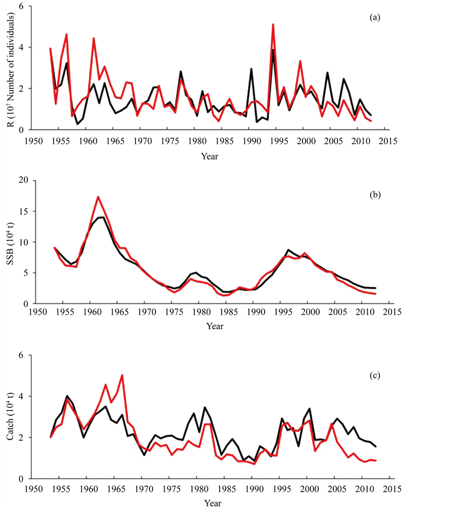
Figure 3. Recruitment (a), spawning stock biomass (b) and catch (c) reproduced by the simulation model (red) and based on ISC data [1] (black).
cases when ln (RPS) was used as the dependent variable. When monthly AO and PDO were only used, i.e., the 24 variables were used as the candidates of environmental factors (Model 1), the selected variables were AO in February, March, April and July, and PDO in March, April, September and October, and the AIC value was −45.10, of which the fitness between the SSB reproduced by the model and the reference value was not good. When the R and SSB of the Japanese sardine were incorporated into the candidate environmental factors (Model 2), the R of the Japanese sardine was added as a variable of the optimal model, and the value of AIC became much smaller (AIC = −63.75). Further, when the modified recruitment of Japanese sardine was used (Model 3), the value of AIC was further improved (AIC = −68.00).
On the contrary, when the SSB of Pacific bluefin tuna was incorporated into the candidate factors (Model 4 or
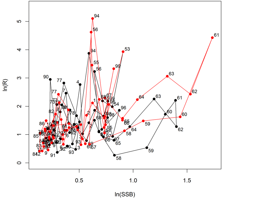
Figure 4. Stock-recruitment relationship reproduced by the simulation model (red) and based on ISC data (black). Figures indicate the year.
5), regardless of whether the R of the Japanese sardine was incorporated or not, the value of AIC became much smaller (AIC = −92.5 or −93.03). Some scientists may consider that this provides clear evidence that a density-dependent effect exists. However, this is really just the illusion of a density-dependent effect. A density-dependent effect can easily explain the important phenomena observed in the population fluctuations; however, it is not a valid explanation as described in detail in the following section.
It is worth emphasizing that when the ln (R) of bluefin tuna was added to the candidate factors instead of ln (SSB) of bluefin tuna (Model 6), the ln (R) of bluefin tuna was chosen as the factor of the optimal model and the resultant optimal model showed much smaller AIC (AIC = −116.38) than that of Model 4 or 5. Therefore, Model 6, which is the model that assumes a positive density-dependent effect by ln (R), was much better than Model 5, which is the usual model to assume a negative density-dependent effect by ln (SSB). However, it does not make sense because the results only indicate that ln (SSB) has a negative relationship to ln (RPS); i.e., ln (SSB) exists in the denominator in ln (RPS), and ln (R) has a positive relationship to ln (RPS); i.e., ln (R) exists in the numerator in ln (RPS). Therefore, when ln (SSB) or ln (R) was added as a candidate factor, the resultant AIC value greatly decreased whether or not the model was valid.
Generally, the same variable in the left side of the equation should not appear in the right-hand side of the same equation. When both the ln (R) and ln (SSB) of bluefin tuna were added as candidate factors (Model 7), both variables were selected as the variables that constructed the optimal model, and the AIC of the resultant optimal model became extremely low (AIC = −2364.98). When this model was applied, the reference and reproduced ln (RPS) values completely coincided with each other. However, the results are a matter of course, because the same values in the left-hand side were used in the right-hand side in equation (11). That is, the minimum AIC does not always indicate a valid model and does not show the validity of the existing of density-dependent effect [9] .
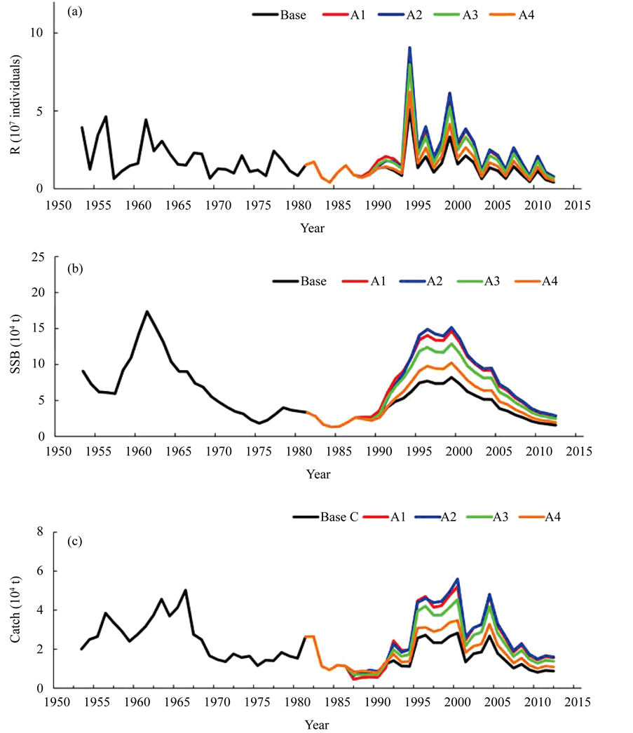
Figure 5. Trajectories of recruitment (a), spawning stock biomass (b) and catch (c) when scenarios A1 to A4 were instituted. The trajectory of the base case (black) was reproduced by the simulation when no regulation was introduced.
The last two models in Table 3 are the cases when ln (R) was used as the dependent variable (Models 8 and 9). Model 8 includes AO by month, PDO by month, the ln (R) and ln (SSB) of Japanese sardine, and the ln (SSB) of bluefin tuna as candidate factors. In this case, AO in February, March and June, and PDO in April, June, July, September and October, and the ln (R) of Japanese sardine were selected as the factors that constructed the optimal model. Importantly, ln (SSB) of bluefin tuna was not selected as a factor that determined the ln (R) of bluefin tuna. Therefore, the fluctuation in ln (R) of bluefin tuna can be explained only by environmental factors, and neither a density-dependent effect by ln (SSB) of bluefin tuna nor a stock-recruitment relationship with the
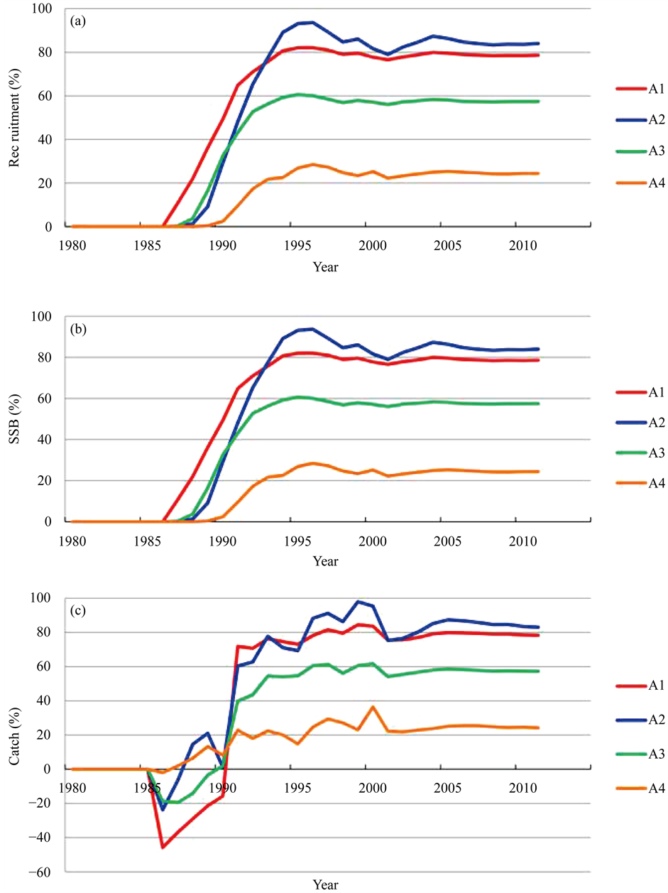
Figure 6. Evaluation of the effect of the regulations instituted for recruitment (a), spawning stock biomass (b) and catch (c) defined by equations (9), (10) and (11), respectively.
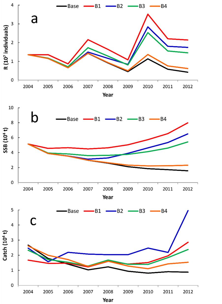
Figure 7. Trajectories of recruitment (a), spawning stock biomass (b) and catch (c) when scenario B1 to B4 were instituted. The trajectory of the base case (black) was reproduced by the simulation when no regulation was introduced.
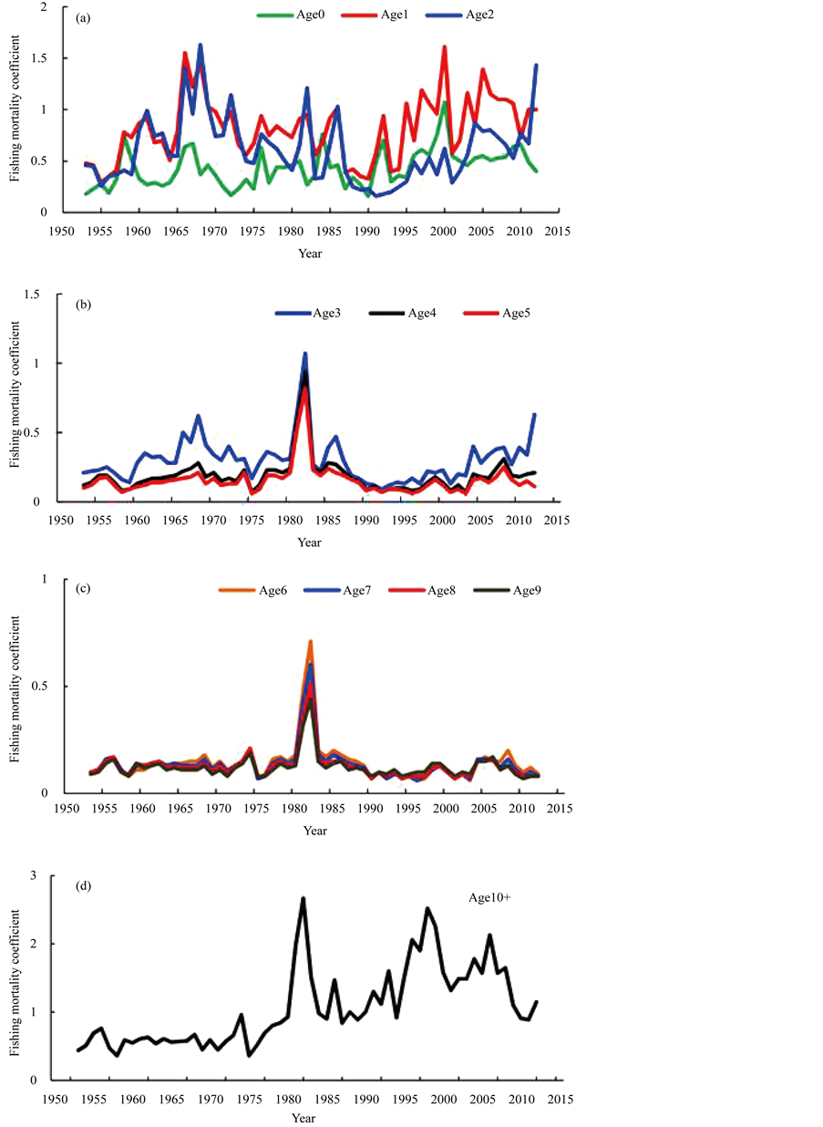
Figure 8. Trajectories of fishing mortality coefficients by age. The fishing mortality coefficients for age 0 - 2 years (a), 3 - 5 years (b), for 6 - 9 years (c), and 10+ years (d) are shown, respectively.
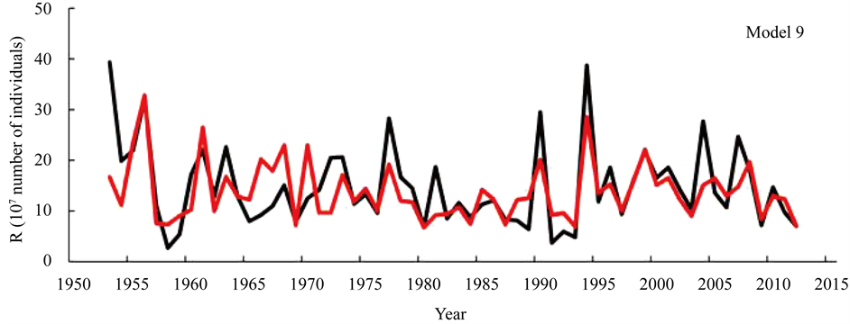
Figure 9. Recruitment reproduced only using the Arctic Oscillation by month, Pacific decadal oscillation by month (model 9) (red) and ISC data [1] (black).
ln (SSB) was detected.
Model 9 was conducted to compare the result of Model 8; i.e., only AO by month and PDO by month were used as candidate factors. In this case, AIC was slightly large compared to Model 8. That is, the ln (R) of bluefin tuna can be well explained only by environmental factors (see Figure 9), and the ln (R) of Japanese sardine was not an indispensable factor. This difference in whether or not the ln (R) of Japanese sardine was chosen as a factor may imply that the fluctuation in the SSB of bluefin tuna has some relation to the ln (R) of Japanese sardine, because the SSB of bluefin tuna exists in the denominator of RPS.
Here, a serious question emerges: namely, which model should we accept as the reasonable model to explain the fluctuation of recruitment? One model uses ln (R) as the dependent variable and the other uses ln (RPS) as the dependent variable. A detailed discussion of this question has already been published by Sakuramoto [10] . He showed that when the function f(.) in equation (1) was cyclically fluctuating, the relationship between ln (R) and ln (SSB) showed one to several loop-shapes, which moved clock-wise or anti-clock-wise depending on the length of the maturity age. Further, when the lengths of maturity age were near half of the cycle of environmental factors, the loop shape did not have a positive or a negative slope. Therefore, in cases where the ln (R) and ln (SSB) seem to have no relationship as with Pacific bluefin tuna, there is a high possibility that cyclic environmental fluctuations are masking the true relationship between ln (R) and ln (SSB). Further, from the biological point of view, a lack of relationship between R and SSB cannot be acceptable. If model 9 expresses the true fluctuation mechanism in R, even if the SSB becomes extremely low in response to incredibly heavy fishing, the recruitment will never change.
In this study, only AO and PDO were used as the physical environmental factors, and R and SSB of the Pacific stock of Japanese sardine were used as biological environmental factors. Other data such as a water temperature over the spawning area and adjacent area, and other indices of physical environmental factors should also be tested as candidate environmental factors.
In this study, the modified recruitment for the Pacific stock of Japanese sardine was used. If reference values of recruitment for the Pacific stock of Japanese sardine were used, the AIC value was little larger (AIC = −63.75) than the case when the modified value was used (AIC = −68.00) as shown in Table 3. This indicates that accurate environmental factors derived from biological relationship are also important to reproduce the RPS. It is, however, difficult to use the long series of biological data for other fish stocks or those of the planktons that the juvenile of bluefin tuna feed upon. If other accurate biological data could be available, the performance of the model could be improved greatly by incorporating them into the present model.
The simulation model that reproduced the R, SSB and catch was extremely sensitive to the given values of natural mortality coefficient, fishing mortality coefficient, mean weight by age and maturity rate by age. As shown in this paper, a slightly smaller natural mortality coefficient reproduced the SSB trends well. However, not only the natural mortality coefficient but also the mean weight by age and maturity rate by age must change year by year. If those detailed and precise information could be made available, the reproduced SSB and catch
Table 4. Results of sensitivity tests when the starting year of regulation was changed.
will explain the fluctuation of the actual ones much better.
In the simulations conducted in this study, the most effective regulation was scenario A2. That is, the effect of the prohibition on age 0 and 1-year-old fishing showed the best performance for recovering the SSB and R. This is because, for Pacific bluefin tuna, the catch number for age 0- and 1-year-old fish has been extremely high (Figure 8), and its ratio to the total catch exceeds 90 percent. This percentage is incredibly high and this indicates that almost all Pacific bluefin tuna are being harvested during very early stages of their development. However, the results were slightly different depending on the year when the regulation was commenced. Table 4 shows the results of sensitivity test of the years of regulation. When the regulation was commenced before 1986, the most effective scenario was scenario A1. These differences would occur depending on the levels of SSB. The level of SSB after 1986 was extremely low, however, the SSB before 1985 was not extremely low (see Figure 3 (b)).
The price for age 0- and 1-year-old fish is low; therefore, regulations to protect juvenile fish might have economic as well as biological merit. However, there are many coastal fishermen who harvest the immature fish of this bluefin tuna. Therefore, when scenario A2 or B2 is chosen for the recovery of this stock, we should carefully consider the effect of the regulation for those fishermen.
5. Conclusions
1) Recruitment per spawning stock biomass of Pacific bluefin tuna can be reproduced using the Arctic Oscillation by month, Pacific decadal oscillation by month and the recruitment number of the Pacific stock of Japanese sardine.
2) Spawning stock biomass could be well reproduced using the simulation model that was constructed with the recruitment per spawning stock biomass and the survival process of population that included the effect of fishing.
3) The effective regulation in the simulations conducted in this paper was a prohibition of fishing for 0- and 1-year-old fish in terms of recovering the spawning stock biomass. The reduction of fishing mortality coefficients for all age fish to 50% of actual values also showed a good performance.
4) The recent reductions of the recruitment and spawning stock biomass appear to be caused by the unregulated harvests, especially for immature fish, since 2004.
Acknowledgements
I thank the Fisheries Agency and Fisheries Research Agency of Japan for providing the recruitment and spawning stock biomass data for the Pacific stock of Japanese sardine. I also thank Drs. Jiro Suzuki, Tokio Wada, Takashi Koya, Naoki Suzuki and Rikio Sato for their useful comments that improved this manuscript.
Cite this paper
Kazumi Sakuramoto, (2016) Case Study: A Simulation Model of the Spawning Stock Biomass of Pacific Bluefin Tuna and Evaluation of Fisheries Regulations. American Journal of Climate Change,05,245-260. doi: 10.4236/ajcc.2016.52021
References
- 1. Pacific Bluefin Tuna Working Group (PBFWG) (2014) Stock Assessment of Bluefin Tuna in the Pacific Ocean in 2014. Report of the Pacific Bluefin Tuna Working Group. International Scientific Committee for Tuna and Tuna-like Species in the North Pacific Ocean. 1-121.
http://isc.fra.go.jp/pdf/2014_Intercessional/Annex4_Pacific%20Bluefin%20Assmt%20Report%202014-%20June1-Final-Posting.pdf - 2. Sakuramoto K. (2013) A Recruitment Forecasting Model for the Pacific Stock of the Japanese Sardine (Sardinops melanostictus) That Does Not Assume Density-Dependent Effects. Agricultural Sciences, 4, 1-8.
- 3. Sakuramoto K. (2014) A Common Concept of Population Dynamics Applicable to Both Thrips imaginis (Thysanoptera) and the Pacific Stock of the Japanese Sardine (Sardinops melanostictus). Fisheries and Aquaculture Journal, 4, 140-151.
- 4. Sakuramoto K. (2015) Illusion of a Density-Dependent Effect in Biology. Agricultural Sciences, 6, 479-488.
- 5. Yatsu A, Watanabe T Ishida M, Sugisaki H, Jacobson LD. (2005) Environmental Effects on Recruitment and Productivity of Japanese Sardine Sardinops melanostictus and Chub Mackerel Scomber japonicus with Recommendations for Management. Fisheries Oceanography, 14, 263-278.
http://dx.doi.org/10.1111/j.1365-2419.2005.00335.x
http://onlinelibrary.wiley.com/doi/10.1111/j.1365-2419.2005.00335.x/abstract - 6. Kawabata J, Watanabe C, Murakami Y, Akamine T, Mito K. (2015) Stock Assessment and Evaluation for the Pacific Stock of Japanese Sardine (Fiscal Year 2015). In: Marine Stock Fisheries Stock Assessment and Evaluation for Japanese Waters (Fiscal Year 2014/2015), Fish Agen and Fish Res Agen Jap, 15-46.
http://abchan.fra.go.jp/digests26/details/2601.pdf - 7. AO (Arctic Oscillation NOAA Climate Prediction Center (2014).
http://www.cpc.ncep.noaa.gov/products/precip/CWlink/daily_ao_index/monthly.ao.index.b50.current.ascii - 8. PDO (Pacific Decadal Oscillation) NOAA’s National Centers for Environmental Information (NCEI) (2014). https://www.ncdc.noaa.gov/teleconnections/pdo/
- 9. Sakuramoto K and Suzuki N. (2012) Effect of Process and/or Observation Errors on the Stock-Recruitment Curve and the Validity of the Proportional Model as a Stock-Recruitment Relationship. Fisheries Science, 78, 41-45.
http://dx.doi.org/10.1007/s12562-011-0438-4 - 10. Sakuramoto K. (2015) A Stock-Recruitment Relationship Applicable to Pacific Bluefin Tuna and the Pacific Stock of Japanese Sardine. American Journal of Climate Change, 4, 446-460.
http://dx.doi.org/10.4236/ajcc.2015.45036