Open Journal of Applied Sciences
Vol.05 No.07(2015), Article ID:58516,10 pages
10.4236/ojapps.2015.57040
Comparison of Loading Functions in the Modelling of Automobile Aluminium Alloy Wheel under Static Radial Load
Samuel Onoriode Igbudu1, David Abimbola Fadare2
1Mechanical Engineering Department, Ambrose Alli University, Ekpoma, Nigeria
2Mechanical Engineering Department, University of Ibadan, Ibadan, Nigeria
Email: samigbudu@yahoo.com, fadareda@yahoo.com
Copyright © 2015 by authors and Scientific Research Publishing Inc.
This work is licensed under the Creative Commons Attribution International License (CC BY).
http://creativecommons.org/licenses/by/4.0/


Received 14 July 2015; accepted 28 July 2015; published 31 July 2015
ABSTRACT
Formulation of exact loading function for radial loading situation has been a major challenge in wheel modeling. Hence, approximate loading functions such as Cosine, Boussinesq, Eye-bar, Polynomial, Hertzian etc., have been developed by different researchers. In this paper, analysis of different loading functions―Cosine (CLF), Boussinesq (BLF) and Eye-bar (ELF) at deferent inflation pressure of 0.3, 0.15 and 0 MPa at specified radial load of 4750N is carried out on a selected aluminium with ISO designation (6JX14H2; ET 42). The 3-D computer model of the wheel is generated and discretised into 3785 hexahedral elements and analysed with Creo Elements/Pro 5.0. Loading angle of 90 degree symmetric with the point of contact of the wheel with the ground is used for ELF, while 30 degrees contact angle is employed for both CLF and BLF. Von Mises stress is used as a basis for comparison of the different loading functions investigated with the experimental data obtained by Sherwood et al while the displacement values (as obtained from the FEM tool) are used as a basis for comparison of the different loading functions, as displacement is not covered by Sherwood et al. Results show that at 0.3MPa inflation pressure, the maximum stress value of CLF approaches the Sherwood value of about 14 MPa and that the CLF function values coincide with Sherwood values at three points along the curve, with values of about 13.8 MPa, 13 MPa and 6.4 MPa at about 0 degree, 15 degree and 20 degree respectively. The BLF value coincides with the Sherwood value at about 18 degree with a magnitude of about 10.6 MPa, while ELF equals the Sherwood value at magnitude of about 6.2 MPa at about 22 degree. At 0.15 and 0 MPa inflation pressure, values CLF, BLF and ELF deviate significantly from the Sherwood values (due to under inflation) with the maximum CLF stress value approaching a value of about 13 and 12MPa respectively. The CLF, BLF and the Sherwood values are the same at about 6 and 3 MPa at 0.15 and 0 MPa inflation pressure respectively. The displacement values for ELF are lesser than those of CLF and BLF for all range of values. The different loading functions values being equal the Sherwood values (used as refernce) at different points, with the CLF having more coincident points along the curve. Higher stress and displacement magnitudes are clustered between 0 degree and about 35 degree. Although, the CLF and BLF offer greater stress and displacement values than ELF, hence the type of loading function adapted for any analysis depends on the type of tyres to be fitted on the wheel. CLF and BLF offers greater prospect for non run flat tyres, while ELF is most suited for run flat tyres. In all cases the right inflation pressure as specified by the tyre manufacture should be employed in any analysis.
Keywords:
Loading Function, Inflation Pressure, Radial Load

1. Introduction
Over the few decades, automobile wheel design has progressively evolved from early spoke designs of wood and steel wheels of the horse drawn carriages and bicycle technology, to flat steel discs and in more recent years to the stamped metal configurations and the newer generation of cast and forged aluminium alloy wheels [1] . Wheel elements, nomenclature, configuration and functions have been described in literature [2] -[6] . The transition from steel to aluminum alloy wheels, and improved shape design for optimum force flux and stress resistance has been reported to reduce weight up to 50, and 16%, respectively [6] -[8] . The style, weight, manufacture and performance are the four main technical issues related to the design of new automobile wheels and/or their optimization. Figure 1 shows the critical technical issues in wheel design [9] -[12] . Advantages of automobile aluminum alloy wheel which include light weight that enhances fuel economy, its noncorrosive characteristics has been widely reported [13] -[15] .
For modern wheel design the determination of optimum wheel design parameters is a very cumbersome and challenging exercise. Analytical methods are known to be complex and strong theoretical background required, while experimental methods are costly, destructive and time consuming. To this effect, application of numerical

Figure 1. Block Diagram of wheel characteristics.
methods such as finite element method (FEM) is currently gaining ground in structural analysis of automobile wheels [16] -[18] . However, in the application of numerical methods, the formulation of appropriate loading function, which describes the actual radial load distribution, representing the vehicle’s and passengers’ weight, on the numerical model has been a major challenge, hence different approximate loading functions ELF, CLF, polynomial and Hetzian functions [2] and BLF [19] -[20] have been developed by different researchers.
1.1. Cosine Loading Function (CLF)
In actual wheel, since a radial load is applied to the wheel on the bead seats with tire, the distributed pressure is loaded directly on the bead seat of the model. The pressure is assumed to have a cosine function distribution mode within a central angle of 40˚ in the circumferential direction, Figure 2 (below).
By using the cosine function accordingly, the distributed pressure, Wr, is given as:
 (1)
(1)
The total radial load, W, is evaluated using Equation (2) as follows,
 (2)
(2)
Substituting Equation (2) into Equation (3) results in,
 (3)
(3)
Integrating,
 (4)
(4)
 (5)
(5)
or solving for W0, gives,
 (6)
(6)
where, rb is the bead seat radius and b is the total width of the bead seats.
1.2. Boussinesq Loading Function (BLF)
This function uses the analogy of a half-plane under the action of concentrated force perpendicular to the boun-
 (a) (b)
Figure 2. (a) loading schematic (b) cosine function loading curve [2] .
dary. For the half plane (Figure 3) the stress function for this problem can be in the form:
 (7)
(7)
Minus sign is chosen because σr obviously will be compressive.
Using Equation (7), we obtain for stresses,
 (8a)
(8a)
 (8b)
(8b)
 (8c)
(8c)
the differential equations and compatibility equation are satisfied identically.
For free upper boundary (stress-free): for ,
,  and
and 
it could be seen that these conditions are satisfied everywhere on line AB, except at point of application of force P.

where,  ;substituting expression for σr gives,
 (9)
(9)
Hence,  and
and
 (10)
(10)
substituting (10) into (8(a)) we have,
 (11)
(11)
1.3. Eye-Bar Loading Function (ELF)
This is based on round rod in an eye bar under an equilibrium of forces as shown in Figure 4 [1] [2] .
 (a) (b)
Figure 3. (a) Loaded half-plane section (b) Half-plane loading curve.
 (a) (b)
Figure 4. (a) Eye-bar loading (b) Eye bar loading curve [2] .
In the Figure 4, r, is the radius of the hole, W is the load imparted, θ, is the angle and qmax is the maximum pointload. The horizontal components of q are balanced. The vertical forces can be related to the external load, W given as:
 (12)
(12)
Defining q = qmaxcosθ and substituting into Equation (12) gives,
 (13)
(13)
Evaluating,
 (14)
(14)
 (15)
(15)
qmax is the unit load N/mm and r is the radius of the bead seat.
The ELF and CLF have been employed in wheel analysis [1] [2] , however, in view of the complexity associated with wheel modeling, no one as at yet defined, accurately, the loading function. It is with this in mind that this study takes to undertake a comparison of the various loading arrangement in order to identify the potentially suited function for wheel design and analysis.
2. Material and Method
A selected automobile aluminum alloy wheel configuration (6JX14H2; ET 42) was used in the analysis. The wheel was sectioned and the cut portions taken to the laboratory to determine the mechanical properties with the aid of a universal testing machine and, chemical properties using the spectrophotometric analysis test. Some of the values obtained-yield stress, poison’s ration and density―form part of the input parameters for the analysis. The actual wheel dimensions were obtained using coordinate measuring machine. The 3-D solid model of the wheel was generated, discretised into elements and analysed with commercially available Finite Element software, PTC® (Creo Elements/Pro 5.0). The model consists of 3785 hexahedral elements. The loading condition for the CLF, BLF and ELF were modeled at different angles (30 and 40 deg for CLF and BLF and 90 deg’ for ELF) and inflation pressure of 0.3 and 0.15 MPa, with a radial load of 4750 N. Figure 5 shows the selected wheel and 3-D computer model.


 (a) (b) (c)
Figure 5. (a) selected aluminium alloy wheel; (b) Computer model of selected wheel; (c) Loaded computer model showing the constraints.
3. Results and Discussion
The mechanical and chemical properties of the wheel material are shown in Table 1 and Table 2 respectively. Results of CLF, BLF and ELF obtained from the FEM simulation were compared with experimental results obtained by Sherwood et al. [20] . The limiting angle 0 to 40 degrees was used in determining the stress values. The displacement values only for CLF, BLF and CLF were discussed, as displacement was not considered by Sherwood et al. in thier study. Observation showed that at 0.3 MPa and at 4750 N the CLF value coincided with the Sherwood value at about 8 degree, 15 and 20 degree symmetric with the point of contact with the ground, with stress values of about 13.8, 13 and 6.4 MPa, respectively. The maximum stress value for the Sherwood curve occurred at about 5 degree with magnitude of about 14 MPa, while that of the CLF occurred at about 10 degree with magnitude of about 14.2 MPa. Their values at point of contact with the ground are about 13.8 MPa and 9 MPa for Sherwood and CLF respectively. The value of BLF at zero degree contact angle was about 11 MPa. Its value at about 18 degree equals the Sherwood value with a magnitude of about 10.6 MPa, which is about the same value with the CLF at about 13 degree symmetric with the point of contact. The BLF value at about 8 degree equals the CLF value at about 10 MPa. The curve intersects the Sherwood curve at a contact angle of about 22 degree with a value of about 6.2 MPa. All values of the CLF and BLF were higher than the ELF values for all range of contact angle. It was, however, observed that while the Sherwood value approaches 0 MPa as from 35 degree, the CLF, BLF and ELF approaches and flattened out at values of about 7, 8 and 6 MPa respectively (Figure 6).
For an inflation pressure of 0.15 MPa and radial load of 4750 N, the value of the CLF at 0 degree is about 7 MPa, coinciding also with the BLF at that angle and with the Sherwood function value at about 28 degree contact angle with a magnitude of about 5 MPa. The maximum value of the CLF was about 13 MPa at about 4 degree contact angle. It drops in value gradually to about 6 MPa at about 10 degree and flattens out at this value up to about 35 degree. The BLF value coincided with the CLF value at 0 and 5 degree, with a magnitude of about 7 and 7.8 MPa respectively and, gradually approaching the CLF values and up to about 20 degree with a magnitude of about 6 MPa and flattens out up to about 35 degree. The Sherwood, CLF and BLF values coincided at about 27 degree with a magnitude 6 MPa each. The shape of the curve for the ELF at 0.15 MPa was almost a constant horizontal curve with a value of about 3 MPa and peaking to a maximum value of about 4 MPa. Its value coincided with the Sherwood value at about 32 degree. All values of the ELF were lower than both CLF and BLF values (Figure 7).
At 0 MPa inflation pressure the magnitude of the CLF stress value at 0 degree was about 6 MPa, coinciding with that of the BLF, while the peak value of CLF was about 12 MPa at about 4 degree; that of the BLF was about 7 MPa at about 2 degree contact angle. The values of the CLF and BLF coincided with the Sherwood value of about 3 MPa at an angle of about 35 degree, while that of the ELF approaches the Sherwood value at about 0.8 MPa at about 37 degree. The value of the ELF at 0 degree was about 2 MPa and peaks to a value of about 3

Figure 6. Relation between Plots of the loading functions and the Sherwood curve on the Von mises Stress at the inboard bead seat at 0.3 MPa inflation pressure and 4750 radial load.

Figure 7. Relation between Plots of the loading functions and the Sherwood curve on the Von mises Stress at the inboard bead seat at 0.15 MPa inflation pressure and 4750 radial load.

Table 1. Mechanical properties of Alloy wheel.
MPa at about 4 degree symmetric with the point of contact with the ground (Figure 8).
The maximum displacement (deformation) at 3 MPa inflation pressure for the CLF, BLF and ELF at point of contact with the ground were about, 0.45, 0.40 and 0.18 mm respectively. The CLF value drops gradually to about 0.175 mm at an angle of about 50 degree and peaks to a value of about 0.2 mm at about 80 degree and drops gradually again to about 0.10 mm at about 140 degree and, flattened out at this value up to 180 degree. The BLF follow the same trend, dropping gradually to a value of about 0.125 at about 50 degree and peaking to

Figure 8. Relation between Plots of the loading functions and the Sherwood curve on the Von mises Stress at the inboard bead seat at 0 MPa inflation pressure and 4750 radial load.
Table 2. Chemical properties of Alloy wheel.
a value of about 0.15 mm at about 90 degree and then dropping to a value of about 0.1 mm. It coincides with the CLF value at about 140 degree and having the characteristics as for the CLF between 160 and 180 degree. The ELF follows the same trend with lower values and with a maximum displacement, at 0 degree, of about 0.20 mm (Figure 9).
The character and shape of the respective curves for CLF, BLF and ELF at 0.15 MPa and 0 MPa inflation are the same as for those of 0.3 MPa inflation pressure. The maximum displacement for ELF, BLF and ELF at 0.15 MPa inflation pressure were about 0.43 mm, 0.375 and 0.175 respectively (Figure 10), while the maximum displacement values, at 0 MPa inflation pressure were about 0.425 mm, 0. 35 and 0.15 mm were obtained respectively for CLF, BLF and ELF at point of contact with the ground (Figure 11). The deformed wheel is shown in Figures 12(a)-(d).
4. Conclusion
Analysis of different loading functions―CLF, BLF and ELF at deferent inflation pressure of 0.3, 0.15 MPa and 0 MPa at specified radial load of 4750N was carried out on a selected aluminium alloy wheel. Von Mises stress was used as a basis for comparison of the different loading functions investigated with the experimental data obtained by Sherwood et al. while the displacement fields (as obtained from the FEM tool) were used as a

Figure 9. Relation between Loading functions on the VonMises Stress at the inboard bead seat at 0.3 MPa inflation pressure and 4750 N radial load.
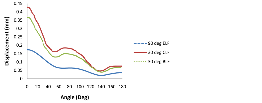
Figure 10. Relation between Loading functions on theVon Mises Stress at the inboard bead seat at 0.15 MPa inflation pressure and 4750 N radial load.

Figure 11. Relation between Loading functions on the Von Mises Stress at the inboard bead seat at 0 MPa inflation pressure and 4750 N radial load.
 (a) (b)
 (c) (d)
Figure 12. Deformed model: (a) front; (b) back; (c) top and (d) bottom.
basis for comparison of the different loading functions as displacement was not covered by Sherwood. Results showed that at 0.3 MPa inflation pressure, the maximum stress value of CLF approaches the Sherwood of about 14 MPa and that the CLF function values coincided with Sherwood values at three points along the curve, with values of about 13.8, 13 and 6.4 MPa at about 0, 15 and 20 degree respectively. The BLF value coincided with the Sherwood value at about 18 degree with a magnitude of about 10.6 MPa, while ELF equaled the Sherwood value at magnitude of about 6.2 MPa at about 22 degree. At 0.15 and 0 MPa inflation pressure, values CLF, BLF and ELF deviated significantly from the Sherwood values (due to under inflation) with the maximum CLF stress value approaching a value of about 13 and 12 MPa respectively. The CLF, BLF and the Sherwood values were the same at about 6 and 3 MPa at 0.15 and 0 MPa inflation pressure respectively. The maximum displacement values were ranked in the following order of decreasing absolute magnitude CLF, BLF and ELF. In other words, the displacement values for ELF were lesser than those of CLF and BLF for all range of values. From the above, it could be said that the different loading functions function values equals the Sherwood values (used as reference) at different points, with the CLF having more coincident points along the curve. Higher stress and displacement magnitudes were clustered between 0 degree and about 35 degree. Although, the CLF and BLF offered greater stress and displacement values than ELF, the type of loading function adapted for any analysis depended on the type of tyre to be fitted on the wheel. CLF and BLF offered greater prospect for non run flat tyres, while ELF was most suited for run flat tyres [2] . In all cases the right inflation pressure as specified by the tyre manufacture should be employed in any analysis.
Cite this paper
Samuel OnoriodeIgbudu,David AbimbolaFadare, (2015) Comparison of Loading Functions in the Modelling of Automobile Aluminium Alloy Wheel under Static Radial Load. Open Journal of Applied Sciences,05,403-413. doi: 10.4236/ojapps.2015.57040
References
- 1. Mohd, I.B.B. Simulation Test of Automotive Alloy Wheel Using Computer Aided Engineering Software. http://umpir.ump.edu.my/143/11. 31/03/11
- 2. Stearns, J.C. (2000) An Investigation of Stress and Displacement Distribution in Aluminium Alloy Automobile Rim. PhD Thesis, University of Akron, Akron.
- 3. Garrett, T.K., Newton, K. and Steeds, W. (2000) Chapter 41 Wheels and Tyres. Journal of Motor Vehicle, 13, 1085- 1108. http://dx.doi.org/10.1016/B978-075064449-5/50042-0
- 4. Kruse, G. and Mahning, F.A. (1976) Comprehensive Methods for Wheel Testing by Stress Analysis. SAE Tecnical Paper Series # 760042. http://dx.doi.org/10.4271/760042
- 5. Muhammet, C. (2010) Numerical Simulation of Dynamic Side Impact Test for an Aluminium Alloy Wheel. Scientific Research and Essays, 5, 2494-2710.
- 6. Raju, R., Satyanrayana, B., Ramji, K. and Suresh, B.K. (2007) Evaluation of Fatigue Life of Aluminium Alloy Wheels under Radial Loads. Engineering Failure Analysis, 14, 791-800. http://dx.doi.org/10.1016/j.engfailanal.2006.11.028
- 7. JISD 4103 (1989) Japanese Industrial Standard. Disc Wheel for Automobiles.
- 8. Kocabicak, U. and Firat, M. (2001) Numerical Analysis of Wheel Cornering Fatigue Tests. Engineering Failure Analysis, 8, 39-54. http://dx.doi.org/10.1016/S1350-6307(00)00031-5
- 9. Tonuk, E., Samim, Y. and Unlusoy, Y. (2001) Pediction of Automobile Tire Cornering Force Characteristics by Finite Element Modelling Analysis. Computers, 1219-1232.
- 10. Carvalho, C., Voorwald, H. and Lopes, C. (2001) Automobile Wheels—An Approach for Structural Analysis and Fatigue Life Prediction. SAE Paper No. 2001-01-4053.
- 11. Kouichi, A. and Ryoji, I. (2002) Shortening Design and Trial Term for Aluminium Road Wheel by CAE. Casting Technology, 74, 533-538. (In Japanese)
- 12. Chang, C.-L. and Yang, S.-H. (2009) Simulation of Wheel Impact Test Using finite Element Method. Engineering Failure Analysis, 16, 1711-1719.
http://dx.doi.org/10.1016/j.engfailanal.2008.12.010 - 13. Baeumel, A. and Seeger, T. (1990) Materials Data for Cyclic Loading. Elsevier Service, Amsterdam.
- 14. Shang, R., Li, N., Altenhof, W. and Hu, H. (2004) Dynamic Side Impact Simulation of Aluminium Wheels Incorporating Material Property Variations, Aluminum. The Minerals, Metals & Materials Society.
- 15. Blake, A. (1990) Practical Stress Analysis in Engineering Design. McGraw-Hill, New York, 363-367.
- 16. Wang, X.F. and Zhang, X.G. (2010) Simulation of Dynamic Cornering Fatigue Test of a Steel Passenger Car Wheel. International Journal of Fatigue, 32, 434-442.
- 17. Reipert, P. (1985) Optimization of an Extremely Light Cast Aluminum Alloy Wheel Rim. International Journal of Vehicle Design, 6, 509-513.
- 18. Mizoguchi, T., Nishimura, H., Nakata, K. and Kawakami, J. (1982) Stress Analysis and Fatigue Strength Evaluation of Sheet Fabricated 2-Piece Aluminum Alloy Wheels for Passenger Cars. Research & Development, 32, 25-28.
- 19. Sakyaan, V. and Lectuere, G. (2006) Note on Theory of Elasticity. Department of Mechanical Engineering, Federal University of Technology, Minna.
- 20. Sherwood, J.A. and Fussel, B.K. (1995) Study of the Pressure on an Aircraft Tire-Wheel Interface. Journal of Aircraft, 32, 921-928.