ABSTRACT

We examine through the lens of dynamical systems a “one dimensional” time mapping of emergent VEV from Pre-Planckian space time conditions. As it is, we will from first principles examine what adding acceleration does as to the HUP previously derived. In doing so, we will be trying it in our discussion with the earlier work done on the HUP. not equal to zero, constant, but large would frequently imply which would have three dissimilar real valued roots. And the situation with not equal to zero yields more tractable result for which will have implications for the HUP inequality in Pre-Planckian space-time, and buttresses an analysis of a 1 dimensional “time” mapping for emergent VEV (vacuum expectation values).

Keywords:

HUP, Dynamical Systems

1. First Looking at the 1 Dimensional Issue We Can Be Considering for Analysis. Leading up to dg_tt

We will be following a first principle investigation of initial equations of state for energy density in space-time as given by B. Hu [1] which we write up as follows: Assuming that an energy density, in Pre-Planckian space-time is given by, if we have an averaged out mean frequency for particle production given by.

(1)

The second line of the above is making the approximation that the insides of the first line, are averaged out to a constant, which is defensible in the situation of a Pre- Planckian space-time condition. Secondly, we are assuming in all of this that is the number of “created” particles in k space, in space-time is in terms of a situation for which we are assuming a very narrow range of k values, so we are when looking at the 2^nd line of Equation (2) referencing an averaged out value for the number of created particles which we then identify as, and have, i.e. with Planck length.

If so, then we could define having a net energy as given by [1]

. (2)

We have several different ways to address what is meant by this energy. Our supposition is that we could make a reference, here, to, if c (speed of light) = 1, to have, here, initially, a transfer of gravitons, as an information carrier, from a prior universe to our present universe so that as a result of a match up in Pre-Planckian space-time to Planckian space time we would have Equation (2) as rendered by, using Hu again, [1] .

(3)

And a graviton count, in the Pre-Planckian era we would give as [1] .

(4)

Here, we would have that would be the “average” number of particles produced in the kth mode, and this kth mode would be in Pre-Planckian space-time. Then combining Equation (3) and Equation (4), if we wish to obtain a “Bose” representation of “gravitons” produced in the immediate aftermath of as the number of particles produced via a VEV, then we would have, if we have.

(5)

Then there would be the rough equivalence given of, say:

We will from here, state that this initial graviton production say for a Planck instant of time would be of the order of 10⁵, so as to have, then if the temperature becomes

. (6)

If

(6a)

Then, the above reduces to the form of equivalencies which we will write up as follows, which will be accessed toward the end of this article.

(6b)

Becomes

(6c)

If one has a grasp of the number of VeV quasi particles where would be the “average” number of particles produced in the kth mode of Pre-Planckian space- time physics, then this would put restrictions on the Pre-Planckian frequency, which we would call [1] .

Our assumptions are that then we would have a way to, get bounds on From Equation (6), which would be then roughly equivalent to initial graviton frequencies, in the onset of the Planckian physics era.

Our last part of information, using Hu again [1] - [3] is in picking the mass of a heavy graviton to be of the order of. From specifications so give, we can isolate

. (8)

Also the mass of [2] [3]

. (9)

We are then ready after some additional work to apply our HUP for Pre-Planckian metric tensor and to determine admissible.

2. Introduction to the Friedman Problem and Also the HUP Connected with Metric Fluctuation

We will be examining a Friedmann equation for the evolution of the scale factor, using explicitly one case being when the acceleration of expansion of the scale factor is kept in, and the intermediate cases of when the acceleration factor, and the scale factor is important but not dominant. In doing so we will be tying it in our discussion with the earlier work done on the HUP but from the context of how the acceleration term will affect the HUP, and making sense of [2] .

(10)

Namely we will be working with [2]

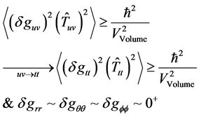
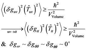
(11)

i.e. the fluctuation dramatically boost initial entropy. Not what it would be if. The next question to ask would be how one could actually have by [4] which if we have the limit of this approaching one, to take into account [2] [4] .

(12)

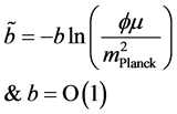
In short, we would require an enormous “inflation” style valued scalar function, and. How could be initially quite large? Within Planck time the following for mass holds, as a lower bound [2] [5] [6] .

(13)

Then by [2] [7]

. (14)

3. How Could Anyone Get the Acceleration of the Universe Factored into Our Scale Factor?

Begin looking at material from page 483-485 of [8]

. (15)

Then, consider two cases of what to do with the ration of and solve the above as a cubic equation.

1) Solutions for Equation (15), in Cubic form for Equation (15) gained by NOT abandoning

Following [2] [8] [9] look first at

(16)

Our approximation is, to set as a constant, but not zero. If so then set

as a non-dimensional but very large quantity. Then a solution exists as given as for a reduced cubic version of Equation (15) which can be given by modifications as presented in this document. i.e. we are using material as given in [9] repeatedly as to solutions to the generalized cubic equation.

Our approximation is, to set as a constant, but not zero. If so then set

as a non-dimensional but very large quantity. Then a solution exists as given as for a reduced cubic version of Equation (15) which can be given by [9]

(17)

And

(18)

And when is set as a non-dimensional constant quantity and possibly quite large, then

. (19)

If so then

. (20)

If is constant and very large, the results of the sign of Equation (20) are as follows [9]

(21)

Here, with very large constant initial we have that the third outcome is by far most likely to happen, in contrast to what would happen in the situation with.

This means that in terms of Equation (21) especially if we have three unequal roots, for Equation (19) that the choice is, in acceleration for a chaotic environment [10] .

4. What Is the Argument against the Usual Heisenberg Uncertainty Principle?

Using [4] and take the limit of the variation to approach 1, then what do we get?

(22)

In short, we would require an enormous “inflation” style valued scalar function, and. i.e. assuming a quantum “bounce” with, but not zero, so as to have Equation (11) render the usual Heisenberg uncertainty principle, would require a scalar value initially of almost infinite value, and there is no reason this would occur. i.e. what we will attempt to do is to model inputs from what can be deduced via deconstructing the super symmetric models, as so beloved by the physics community.

4.1. The Problem with Nearly Infinite Scalarfields Which Shows up in Super Symmetric Models

Going to Kolb, Pi, and Raby, [11] we outline certain problems with the usual SUSY models which in effect argues strongly against a scalar value initially of almost infinite value. The target of what we are examining is an old but still referenced model of inflation in the case of a super symmetric potential of the form of a VEV, which is what we should be considering, namely, if we use a scalar value of a Higgs field, with

. (23)

With a minimum value for Equation (23) according to the first derivative, , if is the super symmetry breaking scale, and

(24)

(25)

With a minimization of a SUSY style Equation (23), and Equation (26) below if. The contention we have is that if one wanted to have Equation (22) satisfied, that with the scale factor ALMOST zero, but not zero, that there is no way to have, and to keep fidelity with the usual HUP relationships of change in energy times change in time as greater than or equal to h bar. Here is the [11] provided SUSY potential for a vanishing VeV.

(26)

i.e. this is still, with some tweaking a commonly accepted SUSY VeV model, with a minimum if, and due to Equation (22) we can argue pretty straight forwardly, that if that the variation in the Pre-Planckian metric as brought up in Equation (22) will NOT allow for the resumption of the usual HUP. So, will in the Pre-Planckian regime, break down. We will next then consider what to expect if there is a dynamical systems treatment for an emergent VeV and what this says physically.

5. Treating Our Problem via Dynamical Systems Ideas

We will first of all, look at the inner dynamics of the metric tensor fluctuation. To do this we encompass the following background. We will next discuss the implications of this point in the next section, of a non-zero smallest scale factor. Secondly the fact we are working with a massive graviton, as given will be given some credence as to when we obtain a lower bound, as will come up in our derivation of modification of the values [2] .

(27)

The reasons for saying this set of values for the variation of the non metric will be in the 3^rd section and it is due to the smallness of the square of the scale factor in the vicinity of Planck time interval.

Begin with the starting point of [12] [13]

. (28)

We will be using the approximation given by Unruh [12] [13] , of a generalization we will write as

(29)

If we use the following, from the Roberson-Walker metric [14] .

(30)

Following Unruh [12] [13] , write then, an uncertainty of metric tensor as, with the following inputs

. (31)

Then, if

(32)

This Equation (32) is such that we can extract, up to a point the HUP principle for uncertainty in time and energy, with one very large caveat added, namely if we use the fluid approximation of space-time [14] [15] .

(33)

Then [2]

. (34)

Then, Equation (32) and Equation (33) and Equation (34) together yield

(35)

How likely is? Not going to happen. See Equation (12) for most discussions.

5.1. How We Can Justifying Writing Very Small 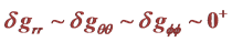Values

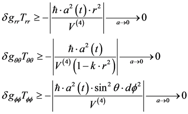
To begin this process, we will break it down into the following coordinates. In therr, θθ and coordinates, we will use the Fluid approximation, [2] with

(36)

If as an example, we have negative pressure, with T_rr, T_θθ and, and, then the only choice we have, then is to set, since there is no way that is zero valued. Having said this, the value of being nonzero, will be part of how we will be looking at a lower bound to the graviton mass which is not zero. We now show how we can frame.

5.2. Considering Now the Reach of Dynamical Systems into This Problem. For δg_tt

We will next be considering the role of a possible dynamical systems mapping upon this problem. To begin with, we will be looking at the role of from a dynamical systems stand point. Now what is meant by a dynamical systems treatment? To begin with we will be looking at the change in a Pre-Planckian metric component as iterated via as a function of time. For the sake of the iterative mapping, we will be looking at if we set.

(37)

What is in Equation (37) shows from inspection that there is, defacto a 1 dimensional mapping for an initially three dimensional process, which is furthermore reflected in what is written up as of the frequency via the following, namely look at if, then Equation (6a) to Equation (6c) lead to the following, namely, if is the number of gravitons produced right after the end of Pre-Planckian space-time, and if is the number of Pre-Planckian “particles” possibly from transit from a prior universe to the present, with say a to be found proportionality factor, then if.

(38)

This can be put into Equation (37). A more conservative treatment of the above,

would be to write a constant, which would put severe restrictions upon

in Pre-Planckian space to write.

(39)

If so, then there would be an iterative map looking like

(39a)

Given this iterative mapping, we can then state clearly its relationship to the Alexan- drov theorem, 1942, which the author was able to ascertain on January 29^th at the Stony brook University weekly talk on Dynamical systems. What we heard is, simply, is that from this talk, that if we ask the following, namely:

Consider a Riemannian metric on of positive sectional curvature. Then is the metric embeddable in? Yes, and here is the theorem to prove it.

Theorem: Alexandrov, 1942:

Suppose is equipped with an intrinsic metric, d, of nonnegative curvature, then is isomorphic to the boundary of a compact, convex set in. (i.e. the picture is to think of the maximum square area of a disc intersecting a sphere in).

i.e. see http://fillastre.u-cergy.fr/wp-content/uploads/2011/04/moscow-fillastre.pdf

The long and short of it is, that if we look at a quantum bounce “ball” of infinitely small radii, but not a point in space, that the relation given in Equation (39a) will define a metric fluctuation, which will be at most a 2 dimensional effect, upon a wave front, most likely embeddable in, of an compact space, here, as we assume, a quantum mechanically generated frequency, for these Gravitational waves, as given by for a front of gravitational waves, composed of gravitons of the frequency, with in this sense being the number of gravitons in the quantum bounce sphere for the Pre-Planckian physical state, and being a geodesicfluctuation of an compact space. We can a priority also assume that the N as given in Equation (39a) is a finite number of iterated steps, which will then lead us to our next discussion which is how and why the usual treatment of early universe conditions, i.e. by the Calabi-Yau construction has issues which are avoided by judicious use of Equation (39a) above.

5.3. Looking at the Calabi-Yau Idealization of Early Universe Conditions and Equation (39a)

A singular manifold Calabi-Yau determines the physical characteristics of the topological soliton states that are interpreted as particles in high energy physics. i.e. what we are doing is when considering the graviton as a particle wave duality, in the formation of Equation (39a) and in doing so, we have to face up to the fact, that the gravitons, in string theory, and the Chalabi Yau setting are almost always massless. i.e. in addition, it is next to impossible for there to be any massive gravitons, since gravitons in this setting as given by [16] - [19] are almost always massless excitations of strings. Not only are we shorn of the geometric insight of the Alexandrov, 1942 theorem, [20] but we are also denied access to the visualization of the quantum bounce as provided by Bojowald, [21] in Nature, as of 2007, and assumed in this document as well as [22] . i.e. the Calabi Yau idealization depends upon massless particles for.

6. Lower Bound to the Graviton Mass Using Barbour’s Emergent Time

In order to start this approximation, we will be using Barbour’s value of emergent time [8] [9] restricted to the Plank spatial interval and massive gravitons, with a massive graviton [10]

. (40)

Initially, as postulated by Barbour [5] [6] , this set of masses, given in the emergent time structure could be for say the planetary masses of each contribution of the solar system. Our identification is to have an initial mass value, at the start of creation, for an individual graviton.

If we can arrive at the identification of

. (41)

Key to Equation (41) will be identification of the kinetic energy which is written as. This identification will be the key point raised in this manuscript. Note that [2] raises the distinct possibility of an initial state, just before the “big bang” of a kinetic energy dominated “pre-inflationary” universe. i.e. in terms of an inflation [2] . The key finding which is in [2] is, that, if the kinetic energy is dominated by the “inflation” that

(42)

This is done with the proviso that w < −1, in effect, what we are saying is that during the period of the “Planckian regime” we can seriously consider an initial density proportional to Kinetic energy, and call this K.E. as proportional to [2]

. (43)

If we are where we are in a very small Planckian regime of space-time, we could, then say write Equation (43) as proportional to [2] , with initial degrees of freedom, and T the initial temperature as low Just before the onset of inflation. The question to ask, then is, what is the value of the initial degrees of freedom, and what is the temperature, T, at the start of expansion.

7. Conclusion. Considering Einstein Space, and Further Research Questions

A way of solidifying the approach given here, in terms of early universe GR theory is to refer to Einstein spaces, via [14] [23] as well as to make certain of the Stress energy tensor [15] as we can write it as a modified Einstein field equation. Then, is given as a constant.

(44)

Here, the term in the Left hand side of the metric tensor is a constant, so then if we write, with R also a constant [24] .

(45)

So as to recover, via the Einstein spaces, the seemingly heuristic argument is given above. Furthermore when we refer to the Kinetic energy space as an inflation [2] , we can also then utilize the following operator equation for the generation of an “inflation field” given by the following set of Equations [25] .

(46)

In the case of the general elliptic operator K if we are using the Fulling reference, [26] in the case of the above Roberson-Walker metric, with the results that the elliptic operator, in this case become,

(47)

Then, according to [26] , if R above, in Equation (47) is initially a constant, we will see then, if m is the inflation mass, that

(48)

Then as an unspecified, for now constant will lead to a first approximation of a Kinetic energy dominated initial configuration, with details to be gleaned from [14] [15] [26] to give more details to the following equation, R here is linked to curvature of spacetime, and m is an inflation mass, connected with the field with the result that

. (49)

If the frequency, of say, Gravitons is of the order of Planck frequency, then this term, would likely dominate Equation (49). More of the details of this will be worked out, and also candidates for the will be ascertained, most likely, we will be looking the Rindler Vacuum as specified in [18] [27] as well as also details of what is relevant to maintain local covariance in the initial space-time fields as given in [19] [28] . Why is a refinement of Equation (49) necessary?

The details of the elliptic operator K will be gleaned from [14] [15] [26] whereas the details of inflation [2] are important to get a refinement on the lower mass of the graviton as given by the right hand side of Equation (41). We hope to do this in the coming year. The mass, m, in Equation (49) for the inflation, not the Graviton, so as to have links to the beginning of the expansion of the universe. We look to what Corda did, in [29] for guidance as to picking values of m relevant to early universe conditions.

It is important to note, that the proper evaluation of Equation (49) will permit, once the role of gravitons in the changing of an inflation contribution is thoroughly experimentally vetted for us to analyze if the criteria raised in [30] are satisfied. As well as understanding the scalar-tensor theories of gravity which are alluded to, in [30] , which have to be either falsified or confirmed. Finally note that what we are doing is an extension of [31] , i.e. GW are experimentally confirmed, and it is necessary to pay attention to the issue of stochastic contributions to signal noise.

i.e. quote:

Binary black hole systems at larger distances contribute to a stochastic background of gravitational waves from the superposition of unresolved systems.

End of quote.

Thoroughly understanding the role of Equation (49) has to be done as to avoid a similar issue here, especially when the emergence of the inflation, as presupposed may significantly add to stochastic noise.

Acknowledgements

This work is supported in part by National Nature Science Foundation of China grant No. 11375279.

Cite this paper

Beckwith, A.W. (2016) Gedanken Experiment for Looking at dg_tt for Initial Expansion of the Universe and Influence on HUP via Dynamical Systems, with Positive Pre-Planckian Acceleration. Journal of High Energy Physics, Gravitation and Cosmology, 2, 531-545. http://dx.doi.org/10.4236/jhepgc.2016.24046

References

- 1. Hu, B. (1984) Vacuum Viscosity and Entropy Generation in Quantum Gravitational Pro- cesses in the Early Universe. In: Fang, L.Z. and Ruffini, R., Eds., Cosmology of the Early Universe, World Press Scientific, Singapore, 23-44.
- 2. Beckwith, A. (2016) Gedanken Experiment for Refining the Unruh Metric Tensor Uncertainty Principle via Schwartz Shield Geometry and Planckian Space-Time with Initial Nonzero Entropy and Applying the Riemannian-Penrose Inequality and Initial Kinetic Energy for a Lower Bound to Graviton Mass (Massive Gravity). Journal of High Energy Physics, Gravitation and Cosmology, 2, 106-124.
http://dx.doi.org/10.4236/jhepgc.2016.21012 - 3. Goldhaber, A. and Nieto, M. (2010) Photon and Graviton Mass Limits. Reviews of Modern Physics, 82, 939-979.
http://arxiv.org/abs/0809.1003
http://dx.doi.org/10.1103/revmodphys.82.939 - 4. Giovannini, M. (2008) A Primer on the Physics of the Cosmic Microwave Background. World Press Scientific, Hackensack. http://dx.doi.org/10.1142/6730
- 5. Barbour, J. (2009) The Nature of Time. http://arxiv.org/pdf/0903.3489.pdf
- 6. Barbour, J. (2010) Shape Dynamics: An Introduction. In: Finster, F., Muller, O., Nardmann, M., Tolksdorf, J. and Zeidler, E., Eds., Quantum Field Theory and Gravity, Conceptual and Mathematical Advances in the Search for a Unified Framework, Birkhauser, Springer-Ver- lag, London, 257-297.
- 7. Handley, W.J., Brechet, S.D., Lasenby, A.N. and Hobson, M.P. (2014) Kinetic Initial Conditions for Inflation. http://arxiv.org/pdf/1401.2253v2.pdf
- 8. Ringstrom, H. (2013) On the Topology and Future Stability of the Universe. Oxford Science Publications, Oxford. http://dx.doi.org/10.1093/acprof:oso/9780199680290.001.0001
- 9. Beyer, W. (1990) CRC Standard Mathematical Tables. 28th Edition, CRC Press, Boca Raton.
- 10. Katok, A. and Hasselblatt, B. (1999) Introduction to the Modern Theory of Dynamical Systems. Cambridge University Press, New York.
- 11. Kolb, E., Pi, S.-Y. and Raby, S. (1984) Phase Transitions in Supersymmetric Grand Unified Models. In: Zhi, F.L. and Ruffini, R., Eds., Cosmology of the Early Universe, World Press Scientific, Hong Kong.
- 12. Unruh, W.G. (1986) Why Study Quantum Theory? Canadian Journal of Physics, 64, 28-130.
http://dx.doi.org/10.1139/p86-019 - 13. Unruh, W.G. (1986) Erratum: Why Study Quantum Gravity? Canadian Journal of Physics, 64, 1453.
http://dx.doi.org/10.1139/p86-257 - 14. Gutfreund, H. and Renn, J. (2015) The Road to Relativity, the History and Meaning of Einstein’s “The Foundation of General Relativity” (Featuring the Original Manuscript of Einstein’s Masterpiece). Princeton University Press, Princeton. http://dx.doi.org/10.1515/9781400865765
- 15. Griffiths, J. and Podolsky, J. (2009) Exact Space-Times in Einstein’s General Relativity. Cambridge Monographs in Mathematical Physics, Cambridge. http://dx.doi.org/10.1017/CBO9780511635397
- 16. http://fillastre.u-cergy.fr/wp-content/uploads/2011/04/moscow-fillastre.pdf
- 17. Morrison, D.R. and Vafa, C. (1996) Compactifications of F-Theory on Calabi-Yau Threefolds (I). Nuclear Physics B, 473, 74-92. http://dx.doi.org/10.1016/0550-3213(96)00242-8
- 18. Morrison, D.R. and Vafa, C. (1996) Compactifications of F-Theory on Calabi-Yau Threefolds (II). Nuclear Physics B, 476, 437-469. http://dx.doi.org/10.1016/0550-3213(96)00369-0
- 19. Klemm, A. and Schimmrigk, R. (1994) Landau-Ginzburg String Vacua. Nuclear Physics B, 411, 559-583. (E-Print arXiv:hep-th/9204060)
- 20. http://www.aei.mpg.de/~theisen/lectures.pdf
- 21. Bojowald, M. (2007) What Happened before the Big Bang? Nature Physics, 3, 523-525.
http://dx.doi.org/10.1038/nphys654 - 22. http://www.nature.com/news/quantum-bounce-could-make-black-holes-explode-1.15573
- 23. Penrose, R. (2010) Cycles of Time: An Extraordinary New View of the Universe. The Bodley Head, London.
- 24. Petrov, A.Z. (1969) Einstein Spaces. Pergamon Press, Oxford.
- 25. Gorbunov, D. and Rubakov, V. (2011) Introduction to the Theory of the Early Universe, Cosmological Perturbations and Inflationary Theory. World Scientific Publishing Pte. Ltd., Singapore.
http://dx.doi.org/10.1142/7873 - 26. Fulling, S.A. (1991) Aspects of Quantum Field Theory in Curved Space-Time. London Mathematical Society Student Texts 17. Cambridge University Press, Cambridge.
- 27. Wald, R.M. (1994) Quantum Field Theory in Curved Spacetime and Black Hole Thermodynamics. University of Chicago Press, Chicago.
- 28. Fredenhagen, K. and Rejzner, K. (2010) Local Covariance and Background Independence. In: Finster, F., Muller, O., Nardmann, M., Tolksdorf, J. and Zeidler, E., Eds., Quantum Field Theory and Gravity, Conceptual and Mathematical Advances in the Search for a Unified Framework, Springer-Verlag, London, 15-23.
- 29. Corda, C. (2012) Primordial Gravity’s Breath. Electronic Journal of Theoretical Physics, 9, 1-10.
http://arxiv.org/abs/1110.1772 - 30. Corda, C. (2009) Interferometric Detection of Gravitational Waves: The Definitive Test for General Relativity. International Journal of Modern Physics D, 18, 2275-2282.
http://dx.doi.org/10.1142/S0218271809015904 - 31. Abbott, B.P., et al. (LIGO Scientific Collaboration and Virgo Collaboration) (2016) Observation of Gravitational Waves from a Binary Black Hole Merger. Physical Review Letters, 116, 061102.
https://physics.aps.org/featured-article-pdf/10.1103/PhysRevLett.116.061102
http://dx.doi.org/10.1103/PhysRevLett.116.061102