Journal of High Energy Physics, Gravitation and Cosmology
Vol.02 No.02(2016), Article ID:65598,27 pages
10.4236/jhepgc.2016.22022
Cosmic Time Transformations in Cosmological Relativity
Firmin J. Oliveira
East Asian Observatory, Hilo, HI, USA

Copyright © 2016 by authors and Scientific Research Publishing Inc.
This work is licensed under the Creative Commons Attribution International License (CC BY).
http://creativecommons.org/licenses/by/4.0/


Received 10 November 2015; accepted 16 April 2016; published 19 April 2016
ABSTRACT
The relativity of cosmic time is developed within the framework of Cosmological Relativity in five dimensions of space, time and velocity. A general linearized metric element is defined to have the form , where the coordinates are time t, radial distance
  for spatials x, y and z, and velocity v, with c the speed of light in vacuum and
  the Hubble-Carmeli time constant. The metric is accurate to first order in
  and
and . The fields
  and
and  are general functions of the coordinates. By showing that
 , a metric of the form
  is obtained from the general metric, implying that the universe is flat. For cosmological redshift z, the luminosity distance relation
  is used to fit combined distance moduli from Type 1a supernovae up to
  and Gamma-Ray Bursts up to
 , from which a value of
  is obtained for the matter density parameter at the present epoch. Assuming a baryon density of
 , a rest mass energy of
  is predicted for the anti-baryonic
  and the
  particles which decay from a hypothetical
  particle. The cosmic aging function
  makes good fits to light curve data from two reports of Type 1a supernovae and in fitting to simulated quasar like light curve power spectra separated by redshift
 . We determine the multipole of the first acoustic peak of the Cosmic Microwave Background radiation anisotropy to be
  and a sound horizon of
  on today’s sky.
Keywords:
Flat Space, Cosmic Time, Time Dilation, Dark Matter

1. Introduction
It has recently been reported [1] on the apparent null effect of cosmic time dilation upon light curve power spectra measurements of some 800 low and high redshift quasars (QSO) monitored for 28 years. This appears to contradict two Supernovae Type Ia (SNe-Ia) light curve evolution studies [2] [3] which show the effect of
broadening of the power spectra time series consistent with a cosmic time dilation of  for redshift z. In
this paper, we show that both the QSO and SNe-Ia results are compatible if account is made for the relativity of cosmic time as developed in the theory of Cosmological Special Relativity (CSR) [4] . We also apply these concepts to fitting the combination of high redshift SNe-Ia distance data [5] and Gamma-Ray Bursts (GRB) data [6] .
The Cosmological Relativity of Carmeli [7] , the general and special theories, is a five dimensional brane world model based on time t, space  and velocity v. It makes only one new assumption, that of the maximum value of cosmic time
  which is the Hubble-Carmeli time constant. In the same way that the constant speed of light c constrains the observations in space and time, so too the constant of cosmic time
  constrains the observations of space and velocity. The familiar Lorentz transformations of Einstein Special Relativity (SR) between observers moving at constant relative velocity v carry over into Cosmological Special Relativity (CSR) between observers separated by relative cosmic time t. And just as in SR, there is the special way that velocities add together which reduces to the Galilean form
  at low velocities with respect to the speed of light, in CSR cosmic times add in an analogous way which has the form
  for low values with respect to cosmic time
  but is modified for larger cosmic times.
In this paper, we derive only the minimum CSR framework we require for the development of cosmic time transformation effects and the luminosity distance relation. We show that for weak fields  and
and  (to be defined below), the universe has a flat, Euclidean geometry. And, due to the additive properties of cosmic time in CSR, this gives us a unique form for the luminosity distance relation. We model cosmic time aging effects in light curve data from SNe-Ia. In comparison to the standard Friedmann-Lemaître-Robertson-Walker (FLRW) model, the CGR luminosity distance relation performs quite well in fits to SNe-Ia and GRB distance data, although it requires more dark matter in the mass density. As a consequence, larger rest masses are predicted for the hypothetical
  particle [8] decay products
  and
and . We also derive a relation for the first acoustic peak of the Cosmic Microwave Background (CMB) anisotropy.
2. The Universe
The five dimensional Cosmological General Relativity of Carmeli [7] is approximated by the linearized metric element,
 (1)
(1)
where
 (2)
(2)
The coordinates are time t, spatials x, y and z and velocity v, with c the speed of light in vacuum and  the Hubble-Carmeli time constant. The linearized model is accurate to first order in
  and
and . The parameter
  is the Hubble constant at zero distance and no gravity and
  where
where  is the
Hubble constant. The fields  and
and  are general functions of the coordinates. The CGR standard value for h is (to three digits) [9] ,
 (3)
(3)
This gives
 (4)
(4)
In Cosmological Relativity the time coordinate is measured backwards from the present at  to the big bang at
 . Just as the speed of light c is the maximum observable speed, the time
  is the maximum observable cosmic time. The gravitational fields are specified by the functions
  and
and . The expansion of the universe occurs when
 (5)
(5)
and it is observed at a specific cosmic time t, so that
 (6)
(6)
Applying (5) and (6) to (1) yields for the expanding universe
 (7)
(7)
which reduces to
 (8)
(8)
The metric (1) defines the Einstein field equations in five dimensions [7] (Sect. 7.3)
 (9)
(9)
where  is the mixed Ricci tensor [7] (Appendix A), R is the Ricci scalar and
  is the mixed energy-momentum tensor, where
  is the effective mass density and
  is the velocity vector. The indices
  for the five dimensions of
 . The Kronecker delta
  for
for , and
, and  for
for . The Carmeli gravitation constant
  where G is Newton's gravitation constant. The
  component of (9) gives us the equation
 (10)
(10)
where
 (11)
(11)
 (12)
(12)
where  and
and . From (10) and (12) we get the Poisson equation for cosmology, in the space-velocity domain,
 (13)
(13)
The effective mass density is defined by
 (14)
(14)
where  is the mass density and
  is the critical mass density. Under the assumption that the mass is uniformly distributed, the mass density
  is independent of the spatial coordinate r, but can depend on time t and velocity v. The critical mass density
  is a constant defined by
 (15)
(15)
It is useful to express the effective mass density as a parameter in terms of the critical mass density. Dividing by  we have
 (16)
(16)
where  is the mass density parameter. For a spatially uniform mass distribution,
  is independent of r, the solution to (13) then takes the form ( [7] , Sect.7.3.2),
 (17)
(17)
where M is an optional point mass centered at the origin of r. Assuming no central mass, we set . Then putting the expression for
  from (17) into (8) and simplifying we get
 (18)
(18)
3. General Solution in Space-Velocity
The integration of (18) over r and v in the space-velocity domain is carried out at a specific time t. We assume that the mass density  is a function of cosmic time only, so that
  will be constant throughout the integration. Substitute
  by (16) and put (18) into the integral form
 (19)
(19)
Integrating (19) and solving for r in terms of v we obtain the general solutions
 (20)
(20)
 (21)
(21)
 (22)
(22)
By use of the identities  and
and , where x is real and
 , we write the general solution as
 (23)
(23)
4. Flat Space Metric
Equation (17) gave the solution for the field . Now consider the solution for the field
  in (1). The
  component of (9) gives us the equation [7]
 (24)
(24)
where
 (25)
(25)
 (26)
(26)
where  and
and . Similar to the case for obtaining
 , we solve (26) to obtain
 (27)
(27)
where M is an optional point mass centered at the origin of r. We see by (17) and (27) that in fact,
 (28)
(28)
and furthermore, that the constants c and  are part of the (cosmological) first term while the constants c and G are part of the (Newtonian) second term. Assuming no central mass (
 ), for the case where the mass density becomes equal to the critical density,
  , from (16), the effective mass density parameter
  and the universe becomes Euclidean.
On the other hand, more generally, we can derive a flatspace metric. Given (28), if we divide (1) by , we can write
 (29)
(29)
where
 (30)
(30)
and
 (31)
(31)
with the condition that
 (32)
(32)
This implies that for weak fields  and
and  we can express the cosmology of the expanding universe in terms of a flat space Euclidean geometry, with a metric of the form
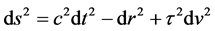 . In the next section we derive this flat space special theory for cosmology.
5. The Cosmological Special Relativistic Transformation
By (29), with notation , we have the metric
 (33)
(33)
where r is given by (31). The expansion of the universe occurs when  and observations are made at a particular instant of time t so that
 . Then for the expansion, (33) gives us
 (34)
(34)
which, upon integration gives the Hubble law
 (35)
(35)
where .
.
In the observable universe there are two classes of objects, those that are bounded by the gravitation of their combined masses and those that are observed to be moving away from one another in the Hubble flow. In other words, if we lump all nearby neighboring galaxies into a super galaxy mass point, then the universe would consist of only super galaxy mass points flying apart in the Hubble flow. Cosmological Special Relativity (CSR) describes these super galactic objects in the universe. However, unlike SR which can have real observers in reference frames which move relatively at less than light speed, in CSR, all galaxies are in the Hubble flow and expand at the Hubble rate h. That is, there are no objects not in the Hubble flow from which to set up a frame of reference and compare observations. Consequently, for CSR we define hypothetical observers in their frames which move relatively at a rate . We derive the transformation of coordinates between these hypothetical frames. However, the coordinates of real galaxies are included in the transformation.
In CSR the age of the universe is , the Hubble-Carmeli time constant, which is assumed to be the same for all cosmic time relative inertial observers and is the maximum cosmic time (just as in SR the speed of light c is the maximum velocity and is constant for all velocity relative inertial observers.) Assume that there are hypothetical observers in reference frames K and
  separated by a fixed cosmic time
 . Each frame is assumed to be unaccelerated (inertial) with respect to cosmic time. Transformations are made between K
describing an object O with “4-vector” coordinates  and
and  describing the same object O with 4- vector coordinates
 . The magnitude of each 4-vector is defined by
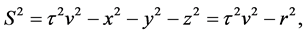 (36)
(36)
 (37)
(37)
with the invariant condition
 (38)
(38)
where  and
and . For the case that object O is a galaxy in the expansion, the invariants
 . We refer to S and
  as 4-vectors even though there are only 2 components, since the 3 spatial components
  are condensed into
 .
.
To obtain the cosmological transformation ( [7] , Sect. 2.2), analogous with the Lorentz transformation, assume that a linear transformation exists between the coordinates of hypothetical frames K and . In frame K define the space-velocity 4-vector
  with magnitude
 (39)
(39)
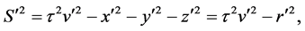
Similarly, in frame  define the space-velocity 4-vector
  with magnitude
 (40)
(40)
By the requirement that the magnitude of a 4-vector is invariant under transformations between reference frames then
 (41)
(41)
Clearly, by (39) and (40), the 4-vectors S and  describe coordinates which can be either in the Hubble flow, when
 , or not in the Hubble flow, when
 . In order to obtain the transformation equations between the 4-vectors it is required that the reference frames K and
  be separated by a fixed cosmic time of
 .
.
Then, for constants  and
and , where
  is a constant hyperbolic angle, define
  and
and  such that
 (42)
(42)
and
 (43)
(43)
To solve for the angle  use the boundary condition
  which represents the origin of frame
 . At
. At  (42) yields,
 (44)
(44)
where
 (45)
(45)
is the fixed cosmic time separating the origins of frame  relative to K. From (44), for
 (46)
(46)
where  is a limiting condition, we use the hyperbolic functional identities to obtain,
 (47)
(47)
 (48)
(48)
Substituting from (47) and (48) into (42) and (43) we obtain
 (49)
(49)
 (50)
(50)
By inverting (49) and (50) we get the inverse transform equations
 (51)
(51)
 (52)
(52)
It can be verified that the transformations (49)-(52) satisfy the invariance requirement of (41) that  by direct substitution into (36) and (37). As was previously mentioned, for a galaxy O with 4-vector
  observed by the observer in frame K, where
 , the transformation Equations (49) and (50)
gives for the galaxy O observed in  the 4-vector
  where, by the invariance of the transformation,
 . Thus, Hubble coordinates are conserved. In the next section we will use this property to obtain the cosmological redshift relation.
6. Cosmological Redshift of Light
We wish to quantify observations of light wave phenomena in the expanding universe made by observers at different cosmic times. Consider the distance r to a galaxy O which is in the Hubble flow, measured by the observer at the origin of K. For the observer at the origin of  the distance to the same galaxy O is
 . If
. If  and
and , where the l’s are the measured wavelengths of the light from the galaxy and N is the fixed number of wavelengths, then taking the ratio of distances we get
 (53)
(53)
where z is the cosmological redshift of the light due to the expansion of space during the cosmic time t between frames  and K. Substituting for r from (51) into (53) gives
 (54)
(54)
 (55)
(55)
For a galaxy which is in the Hubble flow,
 (56)
(56)
Substituting from (56) into (55), and along with (53) yields
 (57)
(57)
Equation (57) is the cosmological redshift of the wavelength of light measured between observers in frames K and . Inverting (57) we get
 (58)
(58)
7. Dilation of Cosmic Time Due to the Expansion of Space
This transformation is similar to the lengthening of the wavelength of light from a distant galaxy by the factor . From the cosmological redshift relation (57) and the fact that the periods
  and
and  of a wave of light are related to the wavelengths
  and
and , respectively, by
 (59)
(59)
 (60)
(60)
we have from (53),
 (61)
(61)
where  and
and . Then the cosmic time dilation from (61) is given by
 (62)
(62)
where we assume that  is an arbitrary time interval in
 .
.
8. Relativity of Cosmic Time
Dividing (51) by (52) we obtain the transformation for the addition of cosmic time from  to K, analogous to the addition of velocities in SR,
 (63)
(63)
where . The inverse transformation, from K to
  is obtained by dividing (49) by (50) giving
 (64)
(64)
where . We refer to (63) and (64) as the general cosmic time addition relations.
Setting  in (63) yields
 (65)
(65)
implying that two cosmic times can never add up to more than . The identical result is obtained from (64) for the time
  when
when .
.
8.1. Contraction of a Small Interval of Cosmic Time in the Past
An increase in cosmic time t by  in frame
  at cosmic time t, where
 , will have a value
  for the observer in K at cosmic time 0 given by the law of addition of cosmic times (63) by setting
  and
and ,
,
 (66)
(66)
which yields
 (67)
(67)
 (68)
(68)
 (69)
(69)
since . This is a cosmic time contraction of a small time
  in
in  at cosmic time t measured by the observer in K [10] . It implies that when viewed from the present epoch, a clock will appear to tick more slowly the further back it is in cosmic time. However, this does not alter the physical constants like G,
  , or e, which remain constants. This is analogous to the case in SR where a clock at the origin of a frame with relative velocity v to the local frame, ticks at the rate
  in its own frame but appears to run more slowly at the rate
 when viewed from the local frame, but the physical constants do not vary.
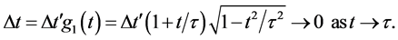
8.2. Dilation of a Small Interval of Cosmic Time in the Present
There is a second kind of effect of time addition which is measured by the observer in  situated at cosmic time t from K. Take the cosmic time lapse
  recorded in K where
 . What is the observation of that time lapse for the observer in
 ? In other words, in
  what is the difference of the later time
  with respect to the earlier time t? The time transformation we use for the
  frame is from (64) by setting
 ,
,  giving
 (70)
(70)
 (71)
(71)
since . This is a cosmic time dilation of a small time interval in frame K measured in
 . It infers that a short time interval at the present epoch corresponds to a larger time interval further back in cosmic time. Note that if
  then (70) gives
  so that we never get a time greater than
  as long as we add times
 .
.
9. Total Cosmic Time Transformation Due to the Expansion of Space and the Additon of Cosmic Times
Combine the two transformations by taking the product of time dilation (62) due to the expansion of the universe with time contraction (69) due to the addition of cosmic times. The total elapsed cosmic time  observed by the observer in K at cosmic time 0 for a small time change
  in frame
  at cosmic time t is given by
 (72)
(72)
where by substituting for  from (57), the cosmic aging function
  is defined by
 (73)
(73)
Substituting for  from (58) in terms of redshift z into (73) yields,
 (74)
(74)
The cosmic aging function  for
for , which gives a time dilation, and
  for
for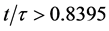 , which corresponds to a time contraction. The maximum occurs at
  where
where  which, from (57), corresponds to a redshift
 . Figure 1 is a plot of the cosmic aging function
 .
.
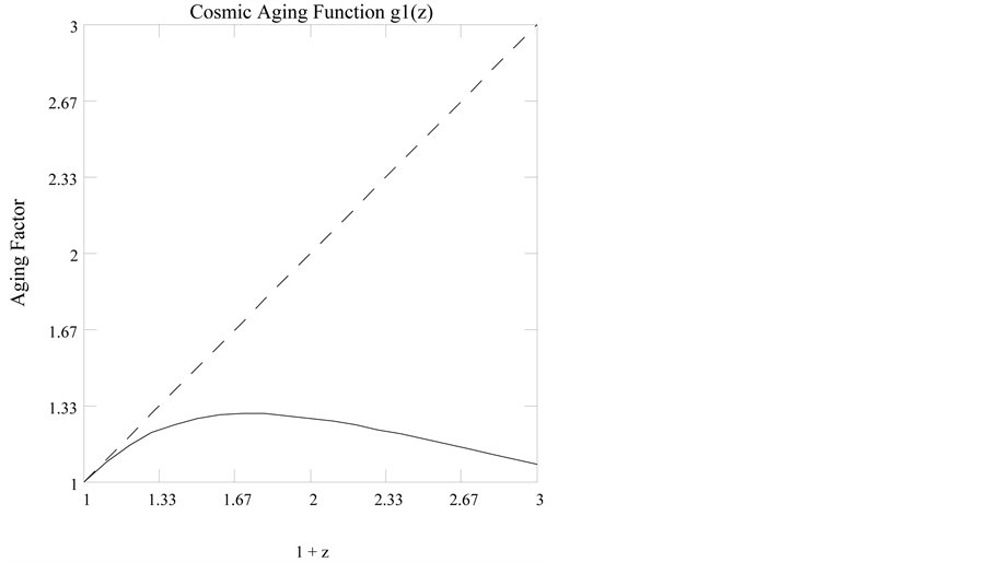
Figure 1. Cosmic aging function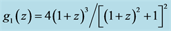 ,
,  , solid line. The dashed line is
 .
.
10. Distances
We use the distance relation (23) with the density , giving
 (75)
(75)
where  is the average mass density parameter at the present epoch.
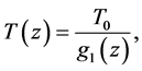
In CGR the luminosity distance relation  includes the contraction of a small interval of cosmic time in the past (69). It enters through the concept that the energy measured over an interval of time
  from a source with luminosity L at rest in frame
  at cosmic time t, radiates a proportional quantity of energy E measured by the observer in K given by
 (76)
(76)
which from (73) is the cosmic aging function  operating on the time interval
 . Using (76) as the form for the energy of the source in the derivation [10] , the luminosity distance
  is given by
 (77)
(77)
which is a factor  of the standard form
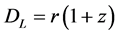 , implying that in CGR sources appear less luminous and thus further away due to the relativity of cosmic time. Substituting for distance r from (75) and for
  from (57), and simplifying, (77) becomes
 (78)
(78)
In practice we make the substitution , [4] (Appendix B. 4.2).
11. Distance Data Fitting
We apply the luminosity distance relation (78) plus a calculated best fit fixed offset  to get the apparent magnitude
  of a distant luminous source,
 (79)
(79)
where we apply (58) to convert from  to z in obtaining
 . We use the CGR standard value [9] of
 . In practice the source absolute magnitude
  is absorbed into the value of the offset
 . We include in our analysis data from both SNE-Ia and GRB studies. The SNE-Ia data come from the Supernova Cosmology Project SCP Union 2.1 data set [5] of 580 SNe-Ia magnitudes and errors up to
 . The GRB distance data of 69 burst events come from [6] which are selected events up to
  from website data provided by [11] . For the
  observed magnitudes and
  respective errors, the
  for the fit is defined by
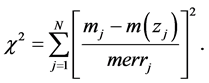 (80)
(80)
The reduced chi-squared  is given by
 (81)
(81)
where N is the number of data samples and k is the number of fitting parameters.
For the  model the luminosity distance relation is given by
 (82)
(82)
where  for flat space [12] .
Although SNE-Ia data are independent of any particular cosmology, this is not so for GRB data which must be calibrated with a specified cosmological model. This is because SNE-Ia have nearby sources to use for calibration, but for GRB there are no nearby sources for this purpose. The original GRB data set was calibrated with the  cosmology. To recalibrate the GRB data for the CGR cosmological model [13] we use the relation
 (83)
(83)
where  is the original GRB distance modulus calibrated with the
  model,
  is the distance modulus calibrated for the CGR model and
  is a conversion factor. The magnitude errors were also converted using (83). We determined a good fitting value of
  which was used to convert the GRB distance moduli for all fits to the CGR model. The converted GRB data were combined with the SNE-Ia
data to form the complete data set. For the CGR model, the number of parameters  for
for ,
,  and
and . The parameter
  is fixed in this analysis, so the number of degrees of freedom
 , the same as for the
  model. The best fit for the CGR model is shown in Table 1 for
  (a conservative estimate of
  error) with offset
  and
and  having a reduced chi-squared
  for
for . The results are shown in Figure 2. Figure
3 shows the histogram of the normalized residual errors for the fit. The solid curve is a Gaussian with mean  and standard deviation
  with an amplitude
  estimated “by eye” to give a close fit to the histogram. The fit appears good [6] [13] [14] .
We fit the  cosmology to the original GRB data set, which was calibrated with
  and
and . We assume
  parameters in the model, for
 ,
,  and
and . We use a fixed Hubble
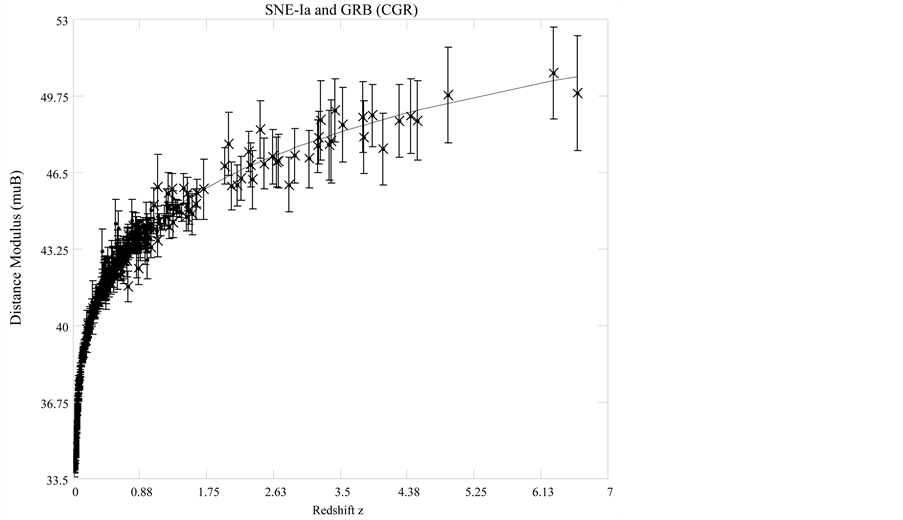
Figure 2. SCP Union 2.1 SNe-Ia data [5] (filled circles) and GRB [6] (dotted x’s). The solid line is for CGR  from (79). The CGR standard value was used for
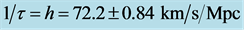 . The parameters for the CGR model were the calculated best fit values, with mass density
 , offset
  and GRB conversion factor
 . Magnitude and magnitude errors both were converted to the CGR model (83). For the fit to 649 data points with 3 parameters the reduced
 .
.
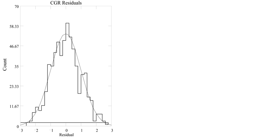
Figure 3. Histogram of CGR residuals  with
with  from (79) with redshift
  from the SCP Union 2.1 SNe-Ia data [5] and GRB data [6] , for calculated best fits with mass density
 , offset
  and
and . The solid line is a standard Gaussian with mean
  and standard deviation
  and the amplitude is scaled by the factor
  to give a good “by eye” fit to the histogram.

Table 1. CGR vs.  model performances with reduced
 . The number of samples
 , and number of parameters
  for both models which gives
 . The CGR row showing the best fit is marked with a (*). Refer to the text for an explanation of the best fitting model. The
  model, with fixed
  and fixed
  has a single best fit for
  based on the original data.
constant of . The best fit occurred for offset
 . Figure 4 shows the Hubble Diagram for the fit of
  to the combined data, with the GRB moduli used unaltered from the
data set. The parameter  is fixed in this analysis, so the number of degrees of freedom is the same as for the CGR model. The reduced chi-squared
 . Figure 5 shows the histogram of the normalized residual errors for the fit. The solid curve is a Gaussian with mean
  and standard deviation
  with an amplitude
  taken from the CGR histogram.
Under the reduced chi-squared statistical model, the ideal reduced  with the errors distributed normally (Gaussian) about
  with
with . The model with a reduced
  which is closest to 1 is preferred. Models with reduced
  are deemed to have too few parameters, so “under fit” the data. Models with reduced
  are deemed to have too many parameters and thus “over fit” the data.
We see that the CGR model under fits the data by , while the
  model over fits the data by
 . For this analysis, the CGR model is
  times better at fitting the combined data. However, considering that we did not vary the mass densities
  and
and , nor the Hubble parameter
 , when fitting with the
  model, we make this conclusion as mainly a statement of our confidence in the CGR model. A more rigorous analysis of the fitting operation would be required.
Dark Matter and the X Particle Hypothesis
Assume that the mass density , that is, composed of baryonic matter
  and cold dark matter
 . For
. For  (95% confidence level) [15] , with the CGR value
 , this gives
 (84)
(84)
Then, for  and
and , the CGR model gives a dark matter density of
 (85)
(85)
compared to the  model which gives a dark matter density of
 (86)
(86)
In an extension to the standard model (SM), a hypothetical X particle [8] is theorized to exist, having 2 species,  and
and  (and their conjugate species
  and
and .) These particles were generated non-thermally during the early universe. The
  decays either into a visible three quark state (UDD), or the hidden state (
 ), with each state having baryon number +1. The conjugate state
  decays to the visible three quark state (
 ) or the hidden state (
 ), with each state having baryon number −1. All of the dark matter today, in
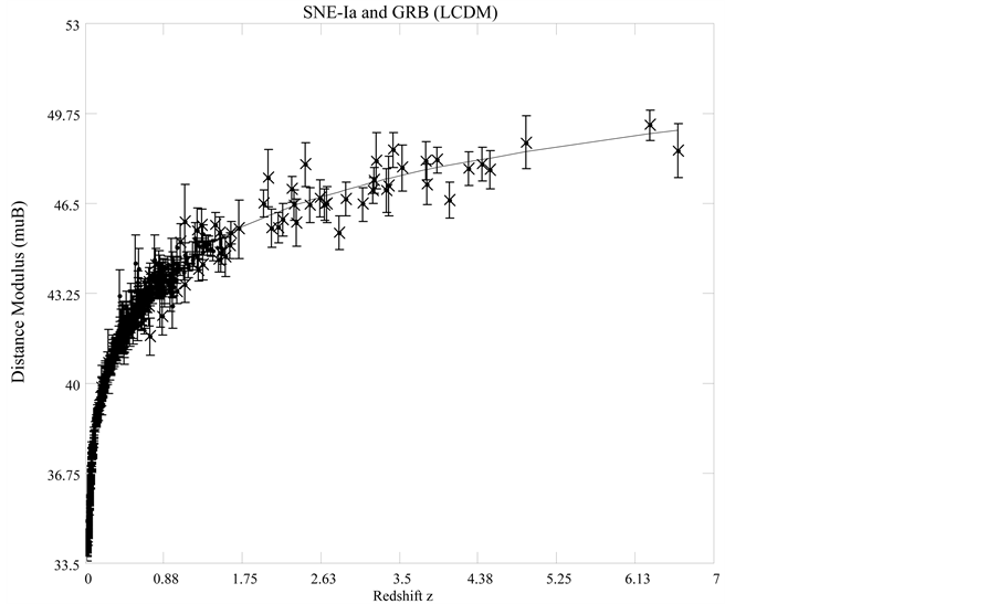
Figure 4. SCP Union 2.1 SNe-Ia data [5] (filled circles) and GRB [6] (dotted x’s). The solid line is for  from (82). The CGR standard value was used for
 . For the
  model, with fixed
  and fixed
 , the calculated best fit value for offset
 . For the fit to 649 data points with 3 parameters the reduced
 .
.
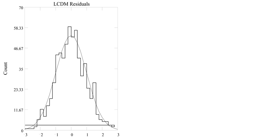
Figure 5. Histogram of  residuals
  for
for  from (82) with redshift
  from the SCP Union 2.1 SNe-Ia data [5] and GRB data [6] , for fixed mass density
  and fixed dark energy mass density
 , with a calculated best fit offset
 . The solid line is a standard Gaussian with mean
  and standard deviation
  and the amplitude factor
  comes from the CGR histogram.
this extended model, is theorized to be composed entirely of hidden particle states ( ). Rare processes can transfer baryonic number from the hidden sector to the visible sector through inelastic scattering of anti-baryonic dark matter states (
 ), annihilating baryons in the visible sector. The cosmic abundance of remnant
  and
and  particles, with densities given by
  and
and , respectively, is the same as the baryon density
  in the universe today, and thus would have the same abundance ratio as
 , the baryon to photon (
 ) ratio. That is,
 (87)
(87)
for a baryon density . Further details of this extension to SM is beyond the scope of this paper. From [8] (Equation (10)) we can relate the ratio of the density of dark matter (anti-baryonic) to baryonic matter in the universe to the ratio of the rest masses of the
 ,
,  and proton by
 (88)
(88)
where  and
and  are, respectively, the
  and
and  particle rest masses and
  is the proton rest mass and we assumed that
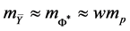 . For the CGR model, (88) yields
 (89)
(89)
which implies
 (90)
(90)
This gives rest mass energies for the  and
and  particles of
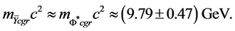 (91)
(91)
For the  model, (88) yields
 (92)
(92)
which implies
 (93)
(93)
This gives rest mass energies for the  and
and  particles [8] of
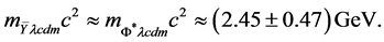 (94)
(94)
In both cases above we have tried to account for the constraint that , where
  is the electron mass, by restricting the range of values to be within
 . This may be only an approximate treatment, at best.
12. Time Dilation in SNe-Ia Light Curves
We now consider two SNe-Ia (SNe) light curve experiments [2] [3] . Common to both experiments is the stretch of the SNe light curve interval for each distant source when compared to the standard nearby (local) source. Because these studies rely on a model for what the light curve looks like in the rest frame of the source SNe, we will require the use of both kinds of cosmic time additions described above. The light curve time interval
 from the distant SNe will be observed to have a time transformation which is a combination of cosmic time addition in the past combined with the time effect of the expansion of space, having the observed value
  which is given by (72),
 (95)
(95)
In CSR this is the time interval that is observed from a source light curve or any time varying phenomenon at a cosmic time t in the past.
On the other hand, we can describe the light curve recorded by the observer in the frame  at cosmic time t relative to our local observer in K at cosmic time 0. A light curve time duration of
  in K, from (71) for a cosmic time addition in the present, corresponds to the value
  in
in  given by
 (96)
(96)
If we make the assumption that
 (97)
(97)
then combining (95) with (97) yields
 (98)
(98)
It is evident that CSR, assuming (97), is consistent with the time dilation reports showing effects of cosmic aging equivalent with  for redshift z. However, to offer a different perspective on cosmic time transformation, we will show plots of the ratio
  given by (95), instead of
  which was used in those reports.
For the SNe data from [2] the light curve agings are given as the light curve width w and the error in the width , obtained directly from [2] (Table 1) for the SCP high z SNe and from [2] (Table 3) for the Calán/Tololo low z SNe. Since the goal of the experiment was to normalize each light curve to a single standard light curve, we
will assume that the equivalent local rest frame time is  which implies from (96) that
 . The reduced observed quantity is
  and we will assume using (98),
 (99)
(99)
We will use (99) to acquire the redshift z and hence  from the light curve rather than using the redshift from the host galaxy. The quantity we use is the ratio
  from (95),
 (100)
(100)
The plotted data are shown in Figure 6. For data points with  the redshift was set to
 . The plot shows the reduction of apparent light curve aging at higher redshift. This is the effect which would be seen in the observed light curve without scaling by the rest frame aging rate. The reduced chi-squared is
  for the data fitted to the cosmic aging rate
 , (74).
The next SNe data are from [3] . We take the aging rates  from [3, Table 3], in the last column, unparenthesized. We compute
 (101)
(101)
The errors come from [3] (Table 3), in the last column, parenthesized. The redshifts are computed from the aging rate data instead of from the given host galaxy values. The plotted data are shown in Figure 7. Again we note the reduction in the aging rate at higher redshifts. The reduced chi-squared for the data fitted to the cosmic aging rate  is
is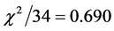 . In Figure 8 we show the combination of all the SNe aging data from the two reports. With 93 total data points the reduced chi-squared is
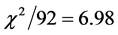 .
.
13. Simulation of Quasar Like Light Curve Power Spectra
The purpose of this section is to simulate quasar like light curve power spectra to compare with the report of observed low and high redshift quasar light curve power spectra [1] . The observed light curve power
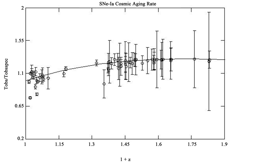
Figure 6. Calán/Tololo low z and SCP high z SNe-Ia light curve time intervals [2] (Goldhaber, et al.). Open circles are  for each of the 58 SNe-Ia. Error bars are computed from the
  data errors. The solid line is the cosmic aging function
  of (74). The reduced
  for the fit of
  to the data is
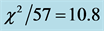 .
.
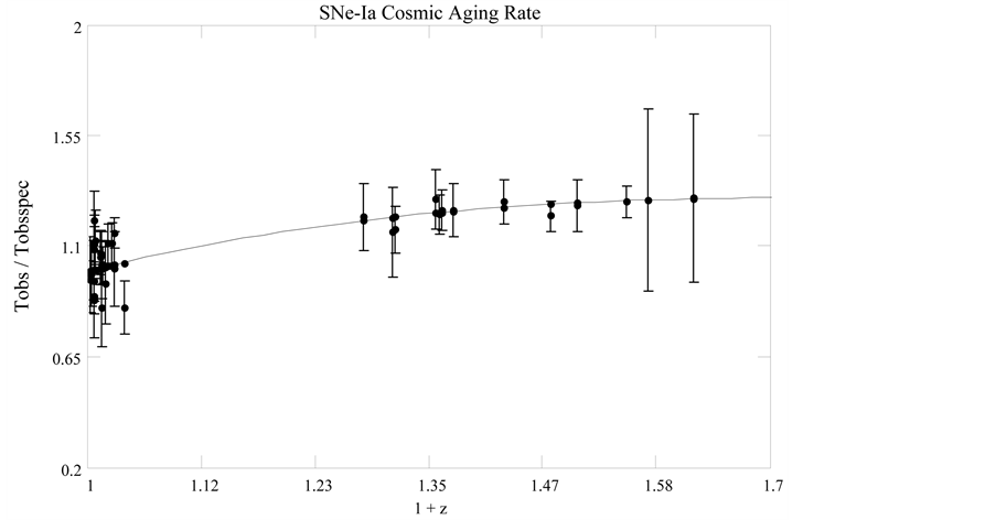
Figure 7. SCP low z and high z SNe-Ia light curve time intervals [3] (Blondin, et al.). Filled circles are  for each of the 35 SNe-Ia. Error bars are computed from the data errors. The solid line is the cosmic aging function
 . The reduced
  for the fit of
  to the data is
 .
.
Figure 8. Combined SNe-Ia light curve time intervals . Open circles are from [2] (Goldhaber, et al.). Filled circles are from [3, Blondin, et al.]. The solid line is the cosmic aging function
 . The reduced
  for the fit of
  to the combined data is
 .
.
spectra [1] (Figure 5, left-hand panel) were found to be identical within the experimental errors. Therefore, we will assume the low and high redshift light curves are identical in the observer frame K. In addition, it is assumed that the redshifts are of pure cosmological origin, with no components of gravitational redshifts or
Doppler shifts. In our simulation, the pseudo quasar light curve apparent magnitudes  at epoch j is generated by the function
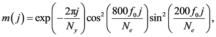 (102)
(102)
for each epoch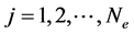 , where
 ,
,  years and
 . The redshifts used are low
  and high
  and
and  are from the quasar time dilation report [1] . For better resolution we used
  instead of the 28 yr which was used in the report. The Fourier power spectrum
  is determined from the magnitudes
  by [1] (Equation (1))
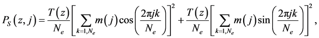 (103)
(103)
where j runs over  equally spaced epochs of simulated data separated by time
 . Then the time transformations will take us from the origin of observer frame K to the quasar rest frame
  at cosmic time t. For CSR the sampling interval
  we use is defined by
 (104)
(104)
where  is given by (74) and
 (105)
(105)
We divide by  in (104) because we are going back in time to the quasar rest frame.
For our purposes, the flat space Friedmann-Lemaître-Robertson-Walker (FLRW) model is the CSR model with the cosmic aging function  replaced by
 . For the flat space FLRW model we use for
 ,
,
 (106)
(106)
where we have again divided out the time transformation to get to the quasar rest frame.
For either model we use the fitting function  defined by [1] , Equation (2)
 (107)
(107)
where  is the power, f is the frequency,
  is the redshift dependent frequency at maximum power and a and b are constants. We use the appropriate form of
  for the CSR or the FLRW models. We show light curve power spectrum plots of
  vs.
vs.  for the light curves at low and high redshift.
Assuming both quasars have identical power spectra in the observer frame K, we obtain the power spectrum from (103) by setting the redshift  which is given by
 . This is shown in Figure 9 with the fitting power function
  parameters
 ,
,  ,
,  where
where  from [1] (Table 1, Observer frame Sample = z < 1, Index = −0.81) and
 . This can be compared with [1] (Figure 5, left-hand panel).
Next we show the light curve power spectra for the low and high redshift quasars,  and
and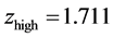 , respectively, as it would be observed in their rest frame. The light curves are corrected by
  since we are obtaining the light curve back in time. We show the quasar power spectrum along with the fitting function
 , which has the same parameters as were used at the origin of K except for the frequency at maximum power which is given by
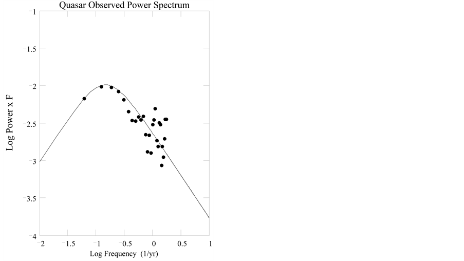
Figure 9. Simulated quasar light curve power spectrum, filled circles, observed at origin of frame K at cosmic time . Low redshift and high redshift quasar power spectra overlap so are shown as one spectrum. The frequency f is
 . The abscissa (horizontal) axis is
  and the ordinate (vertical) axis is
 . Both axes have unit scaling. The function
 , solid line, was fitted iteratively with parameters
 ,
,  ,
,  and
and , yielding
 (108)
(108)
with  from (74). This is plotted in Figure 10. The fitting function has the same parameters for both the low and high redshift spectra as were used in the spectrum at the origin of K except for
 .
.
To show what the power spectra might look like for a flat space FLRW observation we show the low and high redshift quasar light curve power spectra when the light curves are corrected for time dilation by , assuming a flat space cosmology. This is shown in Figure 11. This plot is similar to [1] (Figure 5, right-hand panel). The fitting function
  has the same parameters for both the low and high redshift spectra as were used at the origin of K except for the frequency at maximum power which is given by
 (109)
(109)
In Figure 12 we show a contour plot of the cosmic aging ratio  defined by
 (110)
(110)
between two source fields, one at redshift z and the other at redshift . This is to demonstrate that it is possible to obtain similar aging rates (eg. within 10%) between two sources separated by large redshift. For the above low and high redshifts,
 .
.
For another demonstration of the cosmic aging ratio, we show in Figure 13 the power spectrum for each quasar in its rest frame where  and
and . The aging ratio is
 .
.
14. CMB Anisotropy Acoustic Peak
In CGR the big bang occurred at velocity . At the recombination of protons and electrons in the baryon-photon plasma, when the photons decoupled to form the CMB radiation field, the velocity was
 ,
,
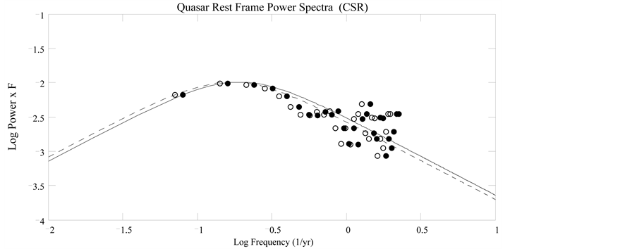
Figure 10. Simulated quasar light curve power spectra in the rest frame  of each quasar where each light curve transforms according to CSR. The frequency f is
 . For the low redshift power spectrum, filled circles,
  , the horizontal axis is scaled by
  with
with  from (74) and the vertical axis has unit scaling. The power spectrum time interval is transformed by
  and the frequency is scaled by
  which effectively sets the scale to unity. For the high redshift power spectrum, open circles,
  , the horizontal axis is scaled by
  and the vertical axis has unit scaling although the power spectrum time interval is transformed by
  and the frequency is scaled by
 . The fitting function
  has the same parameters as used at the origin of K except the central frequency is scaled by
 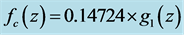 with
with , solid line, and
 , dashed line.
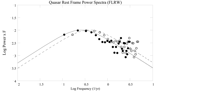
Figure 11. Simulated quasar light curve power spectra in the rest frame  of each quasar where each light curve transforms according to flat space FLRW. The frequency f is
 . For the low redshift power spectrum, filled circles,
  , the horizontal axis is scaled by
 . and the vertical axis has unit scaling. The power spectrum time interval is transformed by
  and the frequency is scaled by
  which effectively sets the scale to unity. For the high redshift power spectrum, open circles,
  , the horizontal axis is scaled by
  and the vertical axis has unit scaling although the power spectrum time interval is transformed by
  and the frequency is scaled by
 . The fitting function
  has the same parameters as used at the origin of K except the central frequency is scaled by
 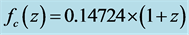 with
with , solid line, and
 , dashed line.
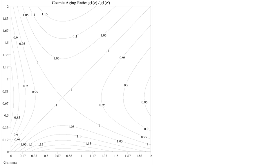
Figure 12. Contour plot of  where
where  from (74). The horizontal and vertical axes are redshift z. Of interest is the curved unity (1) contour going from horizontal lower right to vertical upper left in the graph.
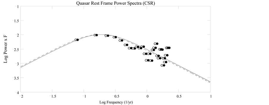
Figure 13. Simulated quasar light curve power spectra in the rest frame  of each quasar, assuming each light curve transforms according to CSR. The frequency f is
 . For the low redshift power spectrum, filled circles,
  , the horizontal axis is scaled by
  and the vertical axis has unit scaling. The power spectrum time interval is transformed by
  and the frequency is transformed by
  which effectively makes the scale unity. For the high redshift power spectrum, open circles,
  , the horizontal axis is scaled by
  and the vertical axis has unit scaling although the power spectrum time interval is transformed by
  and the frequency is scaled by
 . The fitting function
  has the same parameters as used at the origin of K except the central frequency is scaled by
  with
with , solid line, and
 , dashed line.
which is related [4] to the time  of recombination by
 . Applying (58), we have
 (111)
(111)
where  is the cosmological redshift at recombination. The coordinate distance
  to the big bang is given by (23) with
 ,
,
 (112)
(112)
Likewise, the coordinate distance  to the recombination epoch with
 , is given by
 (113)
(113)
We construct a simple model to determine the size of the sound horizon [16] [17] for the longest sound wave, which generates the first acoustic peak. If  is the radius of the sphere of expanding plasma,
  is the average expansion velocity between the big bang and the recombination epoch and
  is the speed of the longest sound wave in the plasma, then, by proportion of velocities,
  is the radius of the sphere containing the longest wave. Assuming that the wave travels along a great circle path of the sphere, the size of the sound horizon
  is given by
 (114)
(114)
Defining , which is the difference of (112) and (113), then from (114), the size of the sound horizon at recombination is given by
 (115)
(115)
The angle  of the sound horizon at recombination is given by
 (116)
(116)
where the angular diameter distance  is given by [10]
 (117)
(117)
where  is the luminosity distance of the recombination epoch. Substituting from (111)-(115) and (117) into (116) and simplifying we obtain
 (118)
(118)
The CMB radiation escaped the matter sphere and expanded to fill all space. The size of the sound horizon  in the CMB on today’s sky is obtained by applying (53) with
 ,
,
 (119)
(119)
Then, the angle  of the sound horizon in the CMB radiation field on today's sky is given by
 (120)
(120)
The multipole l of the first acoustic peak [16] recorded in the CMB radiation field is proportional to the inverse of (120),
 (121)
(121)
Substituting  and
and  into the above equations we obtain a value of
 (122)
(122)
which is in good agreement with observation [18] [19] and,
 (123)
(123)
The size of the sound horizon on today’s sky is , which is 1/5 the value of the standard model.
15. Discussion
Let us review briefly some aspects of the Carmeli five dimensional brane world cosmological model.
15.1. Velocity, Acceleration and Cosmic Distances in CSR
From (33), for  with
with  we have,
 (124)
(124)
This can be manipulated to obtain
 (125)
(125)
where
 (126)
(126)
is the cosmic time (squared). Using (125) this gives for the components of the four-velocity in CSR,
 (127)
(127)
where  and
and
 (128)
(128)
We have from (127) that
 (129)
(129)
 (130)
(130)
Defining  we obtain for the invariant 4-vector length, from (127), (129) and (130),
 (131)
(131)
that is, the length of  is unity in all CSR frames of reference. Multiplying (125) by
 , where
  is the ordinary acceleration measured in the cosmic frame at time 0, the local frame, we obtain after some manipulation,
 (132)
(132)
where
 (133)
(133)
is the acceleration at any cosmic time t. Equation (132) can be put into the form
 (134)
(134)
where
 (135)
(135)
is the velocity of a point which had an acceleration a over a time t. Defining the cosmic distance  we have from (134)
 (136)
(136)
where . This is analogous to the energy equation in SR,
 . Refer to [20] for a thorough treatment of this topic.
15.2. Behavior for Large Cosmic Time
The cosmological redshift (57) and the cosmic aging function (74) are two functions which can be used to describe the behaviour expected at large cosmic time , where
  is the Hubble-Carmeli time constant and is the largest possible time. For the cosmological redshift, for observations of events close to the big bang we have
 137)
137)
The luminosity distance (78), as ,
,  , has the form
 (138)
(138)
For the standard model, the luminosity distance relation, by (137),  , for large t. We see that the CGR luminosity distance, by (138), is larger than the standard model by the factor
 . On the other hand, from the cosmic aging function (73), for an observation
  of an elapsed time
  which occurred close to the big bang time we have
 (139)
(139)
This implies that durations of events, such as for example star formation, star collapse or star bursts, observed in nearby galaxies at cosmic times  (redshifts
 ) should be observed to have shorter durations the further back we look beyond cosmic times
  (redshifts
 ).
).
15.3. The Cosmological Redshift vs. the Cosmic Aging Function
One may ask why the cosmological redshift of the wave length  of light is given by the relation
  instead of with the cosmological aging function
 . The answer is that light wave phenomena do not involve the addition of cosmic times as do evolutionary phenomena such as a star burst or collapse. Light propagation is only affected by cosmic expansion while evolutionary phenomena are affected by cosmic time addition and cosmic expansion.
15.4. The Accelerated Expansion
CGR does not have a cosmological constant, but it does have a critical mass density . From (14), the effective mass density can be defined in terms of a vacuum mass density
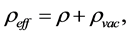 (140)
(140)
where
 (141)
(141)
is the constant negative mass density of the vacuum, which is not the common view of a vacuum density. Differentiating (18) with respect to v we obtain the acceleration in space-velocity, which we put in the form
 (142)
(142)
where
 (143)
(143)
and we have made the substitution, using (141),
 (144)
(144)
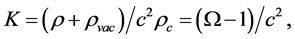
Equation (142) is Hooke’s law of the universe [7, Section 5.4] where K is Hooke’s constant for the universe. If  then K is positive and its solution is a sum of sine and cosine functions and the universe has a decelerated expansion and is closed. If
  then K is negative and the solution is a sum of hyperbolic sinh and cosh functions, which means the universe has an accelerated expansion and is open; this is the situation in our universe today where we derived
 . If
. If  then
then  and the universe is not accelerating and is neither open nor close.
Although beyond the scope of this paper, we give an expression [21] for the vacuum density  in relation to the Bekenstein-Hawking black hole entropy [22] given by
 , where k is Boltzmann’s
constant,  is Planck’s constant over
  and
and  is the area of the event horizon. For our universe of mass
 , where the universe radius is twice the Schwarzschild radius, the entropy is given by
 (145)
(145)
which can be put into the form relating to the vacuum mass density
 (146)
(146)
where the cosmological Planck mass density . The cosmological Planck mass
  and length
 . The value of
 .
.
15.5. Gravitational Waves as a Theoretic Selection Criteria
When gravitational waves are detected we will be able to better quantify the strengths and weaknesses of the standard model (GR) and other models. In this regard, a paper on gravitational wave interferometry [23] has a good description of alternative theories to GR and is a fine starting place for further research. Along those lines of inquiry, [24] describes the behaviour of gravitational waves in Carmeli cosmology, predicting a highly attenuated result for gravitational waves from galactic sources but possible detectability for gravitational waves from within the Milky Way Galaxy.
16. Conclusion
In this paper, we used the linearized approximation of the 5-D Cosmological General Relativity as developed by Carmeli. A flat space CSR model was derived in a general way from the curved space CGR model. The CGR luminosity distance relation was applied to SCP Union 2.1 SNe-Ia distance data up to redshift  combined with GRB distance data up to redshift
 . Utilizing the reduced
  method in the data analysis, it was shown that the CGR model with a best fit mass density of
  performed as well as the
  flat space model with an apriori mass density of
 . Regarding the hypothetical X particle
constituents, the CGR model determines rest mass energies for the  and
and  particles of
  . We also found that CSR could confirm the
  model result of time dilation of
  in SNe-Ia light curves. We also showed how the cosmic aging function
  produced a null effect of time dilation in simulated light curve power spectra between two groups of hypothetical QSO’s separated by a redshift
 . Finally, we gave a model for obtaining the first acoustic peak of the CMB anisotropy, deriving a multipole
 , in good agreement with observation, and with an angle on the sky of
 .
.
Cite this paper
Firmin J. Oliveira, (2016) Cosmic Time Transformations in Cosmological Relativity. Journal of High Energy Physics, Gravitation and Cosmology,02,253-279. doi: 10.4236/jhepgc.2016.22022
References
- 1. Hawkins, M.R.S. (2010) On Time Dilation in Quasar Light Curves. Monthly Notices of the Royal Astronomical Society, 405, 1940-1946. http://dx.doi.org/10.1111/j.1365-2966.2010.16581.x
- 2. Goldhaber, G., Groom, D.E., Kim, A., Aldering, G., Astier, P., Conley, A., et al. (2001) Timescale Stretch Parameterization of Type Ia Supernova B-Band Light Curves. The Astrophysical Journal, 558, 359-368. http://arxiv.org/abs/astro-ph/0104382 http://dx.doi.org/10.1086/322460
- 3. Blondin, S., Davis, T.M., Krisciunas, K., Schmidt, B.P., Sollerman, J., Wood-Vasey, W.M., et al. (2008) Time Dilation in Type Ia Supernova Spectra at High Redshift. The Astrophysical Journal, 682, 724-736. http://arxiv.org/abs/0804.3595 http://dx.doi.org/10.1086/589568
- 4. Carmeli, M. (2002) Cosmological Special Relativity. Second Edition, World Scientific, Singapore.
- 5. Supernova Cosmology Project. 26 January 2016.
http://www.supernova.lbl.gov/Union/figures/SCPUnion2.1_mu_vs_z.txt - 6. Schaefer, B.E. (2007) The Hubble Diagram to Redshift >6 from 69 Gamma-Ray Bursts. The Astrophysical Journal, 660, 16-46. http://www.arxiv.org/abs/astro-ph/0612285 http://dx.doi.org/10.1086/511742
- 7. Carmeli, M. (2008) Relativity: Modern Large-Scale Spacetime Structure of the Cosmos. World Scientific, Singapore.
- 8. Davoudiasl, H., Morrissey, D.E., Sigurdson, K. and Tulin, S. (2010) Unified Origin for Baryonic Visible Matter and Antibaryonic Dark Matter. Physical Review Letters, 105, Article ID: 211304. http://arxiv.org/abs/1008.2399 http://dx.doi.org/10.1103/physrevlett.105.211304
- 9. Oliveira, F.J. and Hartnett, J.G. (2006) Carmeli’s Cosmology Fits Data for an Accelerating and Decelerating Universe without Dark Matter or Dark Energy. Foundations of Physics Letters, 19, 519-535. http://www.arxiv.org/abs/astro-ph/0603500v4 http://dx.doi.org/10.1007/s10702-006-1007-4
- 10. Hartnett, J.G. and Oliveira, F.J. (2007) Luminosity Distance, Angular Size and Surface Brightness in Cosmological General Relativity. Foundations of Physics, 37, 446-454. http://www.arxiv.org/abs/astro-ph/0603500v5 http://dx.doi.org/10.1007/s10701-007-9108-x
- 11. Greiner, J. (22 December 2015). http://www.mpe.mpg.de/~jcg/grbgen.html
- 12. Weinberg, S. (2008) Cosmology. Oxford University Press, New York.
- 13. Hartnett, J.G. (2008) Extending the Redshift-Distance Relation in Cosmological General Relativity to Higher Redshifts. Foundations of Physics, 38, 201-215.
http://arxiv.org/abs/0705.3097 http://dx.doi.org/10.1007/s10701-007-9198-5 - 14. Oztas, A.M. and Smith, M.L. (2014) The Cosmological Constant Constrained with Union2.1 Supernovae Type Ia Data. International Journal of Theoretical Physics, 53, 2636-2661.
http://www.arxiv.org/abs/1401.0724 http://dx.doi.org/10.1007/s10773-014-2061-5 - 15. Burles, S., Nollett, K.M. and Turner, M.S. (2001) Big-Bang Nucleosynthesis Predictions for Precision Cosmology. The Astrophysical Journal, 552, L1-L5. http://www.arxiv.org/abs/astro-ph/0010171
- 16. Cornish, N.J. (2000) Using the Acoustic Peak to Measure Cosmological Parameters. Physical Review D, 63, Article ID: 027302.
http://www.arxiv.org/abs/astro-ph/0005261 http://dx.doi.org/10.1103/physrevd.63.027302 - 17. 11 January 2016. http://astro.uchicago.edu/~frieman/Courses/A411/Lecture8/Lecture8-2010.pdf
- 18. Hinshaw, G., Weiland, J.L., Hill, R.S., Odegard, N., Larson, D., Bennett, C.L., et al. (2009) Five-Year Wilkinson Microwave Anisotropy Probe (WMAP) Observations: Data Processing, Sky Maps, and Basic Results. The Astrophysical Journal Supplement Series, 180, 225-245. http://www.arxiv.org/abs/0803.0732 http://dx.doi.org/10.1088/0067-0049/180/2/225
- 19. Hanany, S., Ade, P., Balbi, A., Bock, J., Borrill, J., Boscaleri, A., et al. (2000) MAXIMA-1: A Measurement of the Cosmic Microwave Background Anisotropy on Angular Scales of 10'-5. The Astrophysical Journal Letters, 545, L5- L9. http://www.arxiv.org/abs/astro-ph/0005123
- 20. Carmeli, M. (2001) Velocity, Acceleration and Cosmic Distances in Cosmological Special Relativity. http://www.arxiv.org/abs/astro-ph/0111260
- 21. Oliveira, F.J. (2012) Particle Pair Production in Cosmological General Relativity. International Journal of Theoretical Physics, 51, 3993-4005.
http://www.arxiv.org/abs/1203.4797 http://dx.doi.org/10.1007/s10773-012-1291-7 - 22. Wikipedia: Black Hole Thermodynamics. http://www.wikipedia.org/wiki/Black_hole_thermodynamics
- 23. Corda, C. (2009) Interferometric Detection of Gravitational Waves: the Definitive Test for General Relativity. International Journal of Modern Physics D, 18, 2275-2282.
http://www.arxiv.org/abs/0905.2502 http://dx.doi.org/10.1142/S0218271809015904 - 24. Hartnett, J.G. and Tobar, M.E. (2006) Properties of Gravitational Waves in Cosmological General Relativity. International Journal of Theoretical Physics, 45, 2181-2190. http://www.arxiv.org/abs/gr-qc/0603067 http://dx.doi.org/10.1007/s10773-006-9181-5