Journal of Applied Mathematics and Physics
Vol.05 No.12(2017), Article ID:81495,9 pages
10.4236/jamp.2017.512196
The Oscillatory Motion of Oldroyd-B Fluid by Incorporating Some of the Mechanical Factors
Amir Khan1, Gul Zaman2, Yongjin Li3*, Saeed Ahmad2, Altaf Hussain1
1Department of Mathematics and Statistics, University of Swat, Khyber Pakhtunkhwa, Pakistan
2Department of Mathematics, University of Malakand, Chakdara, Dir (Lower), Khyber Pakhtunkhwa, Pakistan
3Department of Mathematics, Sun Yat-sen University, Guangzhou, China
![]()
Copyright © 2017 by authors and Scientific Research Publishing Inc.
This work is licensed under the Creative Commons Attribution International License (CC BY 4.0).
http://creativecommons.org/licenses/by/4.0/


Received: September 4, 2017; Accepted: December 26, 2017; Published: December 29, 2017
ABSTRACT
The aim of this paper is to present a numerical study of oscillatory motion of Oldroyd-B fluid in a uniform magnetic field through a small circular pipe. First, we derive the orientation stress tensor by considering the Brownian force. Then, the orientation stress tensor is incorporated by taking Hookean dumbbells on Brownian configuration fields in the Oldroyd-B model. The Oldroyd-B model is then reformulated coupled with the momentum equation and the total stress tensor. Finally, we analyze the orientation stress tensor in the pipe by the numerical simulations of the model and showed that the effect of orientation stress tensor is considerable although the Brownian force is sufficiently small.
Keywords:
Oldroyd-B Fluid, Brownian Force, Finite Difference, Oscillatory Flows

1. Introduction
The theory of Newtonian fluids well enough describes the mechanical behavior of many real fluids. But still we have a lot of fluids which are not properly entertained by Newtonian fluid such as ketchup, blood, paints, shampoo, pulps, honey, oil and drilling mud etc. In general, these fluids are known as non Newtonian fluids. As we know, these fluids are commonly used in daily life and have many applications toward industries as well as to academics. Many researchers have attempted to develop a single model which represents all these fluids but they haven’t found any success in their struggle. Consequently, different fluids model have been proposed for these fluids. Which are commonly divided into three main classes namely, fluids of differential type, integral type and rate type. The rate type models are considered to be much more practical and important. One of the famous rate type model is Maxwell fluids [1] , considered to be the first rate type model. This model is still very attractive for the researchers. Rajagopal [2] formulated a formal thermodynamic framework based on the seminal work of Maxwell, for different class of fluids. Among them is Oldroyd-B model, which is considered to be the more generalized fluid model as it deals with relaxation as well as retardation times. Most of the fluids are particular cases of Oldroyd-B fluid.
In the last few decades, oscillating bodies have widely studied due to importance in practical fields and experiments. They are considered in various biological and industrial processes, for example in nuclear reactor, oil exploitation, the periodicity of blood flow [3] , food industry, bio-engineering and chemistry, cellulose and soap solutions etc. Also, magnetohydrodynamics (MHD) flows plays an important role in development of energy generation and in the dynamics of geophysical and astrophysical fluid. In the last few years researchers contribute alot on MHD flow, see [4] [5] [6] [7] and reference therein.
In this paper, we developed an Oldroyd-B model by taking a total stress tensor which consists of the shear stress tensor, the orientation stress tensor (OST) and isotropic pressure stress tensor. The model deals with the dynamics of oscillatory flow of Oldroyd-B fluid inside a circular pipe. Continuity and momentum equations along with Oldroyd-B model have been taken under consideration. The whole system is then reformulated along with the total stress tensor. Finally, we solve numerically by employing the finite-difference scheme for the Oldroyd-B model and orientation stress tensor. Our numerical results show that in spite the Brownian force is very small still the effect of the orientation stress tensor on the Oldroyd-B model is considerable.
2. Reformulation of Oldroyd-B Model
In this section, we incorporate a Brownian force when MHD flow of Oldroyd-B fluid is passing through a pipe. To do this we consider the orientation stress tensor for time-dependent incompressible flow [3] :
(1)
for some , here is the dumbbell inverse relaxation time, a is the radius of bead, is the temperature, is the Boltzmann constant, is the viscosity of fluid and is the velocity. Equation (1) will be used to reformulate the Oldroyd-B model. Many researchers [8] [9] [10] [11] have developed their models by taking a total stress tensor which consists of the shear and isotropic pressure stress tensors without considering the orientation stress tensor. Here, we extend our model by taking the shear and isotropic pressure stress tensors as well as orientation stress tensor with a constant g (the elastic modulus). Let be the total stress tensor and be the velocity of the MHD flow. For the unsteady incompressible flow the continuity and the momentum equations are given by:
(2)
where , in which the magnitude of a uniform magnetic field is denoted by and the direction of uniform magnetic field is normal to the motion of fluid, is the fluid electrical conductivity, is the density of fluid, is the fluid viscosity, identity matrix is represented by , is the orientation stress tensor, elastic modulus is represented by g and- represents the isotropic pressure stress tensor.
Now, we reformulate the Oldroyd-B model by supposing , , and combining it with the momentum equation and Equation (1)
(3)
where is the material derivative, and represents the material constants.
Let , is the velocity and
(4)
is the orientation stress tensor which is considered to be symmetric [12] - [20] . The total stress tensor consists of nine components are given by
(4a)
To obtain the components of the OST , first we determine all the nine components of the OST from Equation (4) then we solve the reformulated Oldroyd-B model to get all these nine components:
(5)
Here, Kronecker delta is represented by . Pressure p will be obtained by substituting all those nine components of in the momentum equation.
(6)
Then we substitute the OST and the pressure p in Equation (4a) to get the total stress tensor .
3. Total Stress Tensor
To find the numerical solution we use an iterative method. Several mixed and semi-implicit methods have been proposed to get more efficient solvers while preserving stability. We take velocity as
where is the amplitude of the velocity and is the frequency. The appropriate conditions of velocity are:
(7)
where r is the radius of the pipe. For the sake of simplification we neglect some of the components of the OST by taking . Thus, Equation (6) becomes
(8)
Similarly Equation (7) becomes
(9)
To get solution of Equation (6), we need to find the component of OST and pressure p with and without OST.
(10)
To solve the above system we use the following values for different parameters:
, , , , and . The components of total stress tensor can be obtained from the pressure and from the corresponding components of OST. All the nine components of the total stress tensor are given by
(11)
4. Numerical Results and Discussion
Some 3D surfaces are presented here to show the components of OST and the effect of OST on total stress tensor. Figure 1 and Figure 2 shows the components of orientation stress tensor. The component with the configuration of Brownian force is depicted in Figure 1. The components

Figure 1. component of the orientation stress tensor.
and are similar and since S is symmetric so . In Figure 2 we have shown the components . All the remaining components of S are taken to be zero. Figure 1 and Figure 2 shows that all the components of OST are not similar. Figure 3 shows the component of total stress tensor with the OST , which is the numerical result of the system (11). We solve system (11) numerically for component and for pressure p with the OST, and then by putting and p in Equation (5) we get the component of

Figure 2. component of the orientation stress tensor.
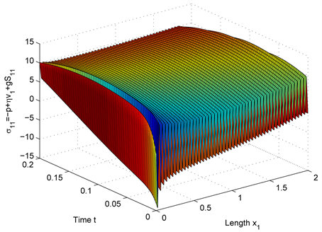
Figure 3. component of total stress tensor with .
total stress tensor with OST. In system (11) in the absence of OST we solve for p, and by substituting it in Equation (5) we get the component of total stress tensor without the OST component and is depicted in Figure 4. In Figure 5 we show the total stress tensor with and without the OST. From the figure it is obvious that inspite the Brownian force is very small still the effect of the OST is

Figure 4. component of total stress tensor without .

Figure 5. with (dotted) and without (solid) at .
considerable. Note that we take only the -axis of velocity for numerical results, which shows that the magnitudes of all of the components of stress are not similar. Hence, from these figures we can examine all the results and can find the impact of total and OST as well as the effect of pressure quantitatively on the phenomena of flow in order to confirm the validity of the said Oldroyd-B model.
Special Cases. The similar solutions for Newtonian, Maxwell and second grade fluids performing the same motion are obtained here as limiting cases of the solutions. In the absence of the OST the Oldroyd-B model in the system (6) is reduced to the following model:
1) Taking and , model for Newtonian fluid is obtained.
2) Taking and , then the model is simplified to Maxwell model.
3) Taking and , the model reduced to second-order fluid.
5. Conclusion
In this article, we presented oscillatory motion of Oldroyd-B fluid in a uniform magnetic field using numerical scheme. The fluid is passing through a small circular pipe. Taken into consideration the Brownian force, we derive the orientation stress tensor. Then, the orientation stress tensor is incorporated by taking Hookean dumbbells on Brownian configuration fields in the Oldroyd-B model. The reformulated Oldroyd-B model has been obtained with the help of momentum equation and the total stress tensor equation. At the end, the orientation stress tensor has been analyzed by the numerical simulations of the model which shows that the effect of orientation stress tensor is considerable although the Brownian force is sufficiently small.
Acknowledgements
This work was supported by the National Natural Science Foundation of China (11571378).
Cite this paper
Khan, A., Zaman, G., Li, Y., Ahmad, S. and Hussain, A. (2017) The Oscillatory Motion of Oldroyd-B Fluid by Incorporating Some of the Mechanical Factors. Journal of Applied Mathematics and Physics, 5, 2402-2410. https://doi.org/10.4236/jamp.2017.512196
References
- 1. Maxwell, J.C. (1866) On the Dynamical Theory of Gases. Philosophical Transactions of the Royal Society, 157, 49-88.
- 2. Rajagopal, K.R. and Srinivasa, A. (2000) A Thermodynamic Framework for Rate Type Fluid Models. Journal of Non-Newtonian Fluid Mechanics, 88, 207-227. https://doi.org/10.1016/S0377-0257(99)00023-3
- 3. Zaman, G., Islam, S., Kang, Y.H. and Jung, I.H. (2012) Blood Flow of an Oldroyd-B Fluid in a Blood Vessel Incorporating a Brownian Stress. Science China Physics, Mechanics and Astronomy, 55, 125-131. https://doi.org/10.1007/s11433-011-4571-y
- 4. Khan, A. and Zaman, G. (2017) Hydromagnetic Flow near an Accelerating Plate in the Presence of Magnetic Field through Porous Medium. Georgian Mathematical Journal. https://doi.org/10.1515/gmj-2017-0017
- 5. Khan, A. and Zaman, G. (2015) The Motion of a Generalized Oldroyd-B Fluid Between Two Side Walls of a Plate. South Asian Journal of Mathematics, 5, 42-52.
- 6. Khan, A. Zaman, G. and Rahman, G. (2015) Hydromagnetic Flow near a Non-Uniform Accelerating Plate in the Presence of Magnetic Field through Porous Medium. Journal of Porous Media, 18, 801-809. https://doi.org/10.1615/JPorMedia.v18.i8.50
- 7. Khan, A. and Zaman, G. (2016) Unsteady Magneto-Hydrodynamic Flow of Second Grade Fluid Due To Uniform Accelerating Plate. Journal of Applied Fluid Mechanics, 9, 3127-3133.
- 8. Pontrelli, G. (2000) Blood Flow through a Circular Pipe with an Impulsive Pressure Gradient. Mathematical Models and Methods in Applied Sciences, 10, 187-202. https://doi.org/10.1142/S0218202500000124
- 9. Pontrelli, G. (2001) Blood Flow through an Axisymmetric Stenosis. Proceedings of the Institution of Mechanical Engineers, Part H: Journal of Engineering in Medicine, 215, 1-10. https://doi.org/10.1177/095441190121500101
- 10. Yeleswarapu, K.K., Kameneva, M.V., Rajagopal, K.R. and Antaki, J.F. (1998) The Flow of Blood in Tubes: Theory and Experiment. Mechanics Research Communications, 25, 257-262. https://doi.org/10.1016/S0093-6413(98)00036-6
- 11. Lee, S.W., Sohn, S.M., Ryu, S.H., Kim, C. and Song, K.W. (2001) Experimental Studies on the Axisymmetric Sphere-Wall Interaction in Newtonian and Non-Newtonian Fluids. Korea-Australia Rheology Journal, 13, 141-148.
- 12. Mekheimer, Kh.S. (2008) Effect of the Induced Magnetic Field on Peristaltic Flow of a Couple Stress Fluid. Physics Letters A, 372, 4271-4278. https://doi.org/10.1016/j.physleta.2008.03.059
- 13. Quarteroni, A. (2006) What Mathematics Can Do for Simulation of Blood Circulation.MOX Report, Jan 16.
- 14. Bellert, S.L. (2001) Computational Fluid Dynamics of the Human Carotid Bifuraction. B. E. Thesis, University of Queensland, Queensland.
- 15. Pries, A.R., Neuhaus, D. and Gaehtgens Freie, P. (1992) Blood Viscosity in Tube Flow: Dependence on Diameter and Hematocrit. American Journal of Physiology, 263, H1770-H1778. https://doi.org/10.1152/ajpheart.1992.263.6.H1770
- 16. Fung, Y.C. (1993) Biomechanics: Mechanical Propreties of Living Tissues. Springer-Verlag, New York. https://doi.org/10.1007/978-1-4757-2257-4
- 17. Song, Y.S. and Youn, J.R. (2004) Modeling of Rheological Behavior of Nanocomposites by Brownian Dynamics Simulation. Korea-Australia Rheology Journal, 16, 201-212.
- 18. Wilson, H.J. (2006) Polymeric Fluid Lecture, GM05 part 1. Jan 9.
- 19. Underhilla, P.T. and Doyle, P.S. (2007) Accuracy of Bead-Spring Chains in Strong Flows. Journal of Non-Newtonian Fluid Mechanics, 145, 109-123. https://doi.org/10.1016/j.jnnfm.2007.05.011
- 20. Everitt, S.L. Harlen, O.G., Wilson, H.J. and Read, D.J. (2003) Bubble Dynamics in Viscoelastic Fluids with Application to Reacting and Non-Reacting Polymer Foams, Journal of Non-Newtonian Fluid Mechanics, 114, 83-107. https://doi.org/10.1016/S0377-0257(03)00108-3