Journal of Applied Mathematics and Physics
Vol.04 No.07(2016), Article ID:69245,17 pages
10.4236/jamp.2016.47145
Filtered Leapfrog Time Integration with Enhanced Stability Properties
Ari Aluthge, Scott A. Sarra, Roger Estep
Department of Mathematics, Marshall University, Huntington, WV, USA
![]()
Copyright © 2016 by authors and Scientific Research Publishing Inc.
This work is licensed under the Creative Commons Attribution International License (CC BY).
http://creativecommons.org/licenses/by/4.0/


Received 27 May 2016; accepted 25 July 2016; published 28 July 2016
ABSTRACT
The Leapfrog method for the solution of Ordinary Differential Equation initial value problems has been historically popular for several reasons. The method has second order accuracy, requires only one function evaluation per time step, and is non-dissipative. Despite the mentioned attractive pro- perties, the method has some unfavorable stability properties. The absolute stability region of the method is only an interval located on the imaginary axis, rather than a region in the complex plane. The method is only weakly stable and thus exhibits computational instability in long time integrations over intervals of finite length. In this work, the use of filters is examined for the purposes of both controlling the weak instability and also enlarging the size of the absolute stability region of the method.
Keywords:
Leapfrog Method, Computational Mode, Weak Stability, Method of Lines, Numerical Weather Prediction

1. Introduction
In this work the stability properties of a well known linear multistep method (LMM) are examined. The method is based on a three point polynomial finite difference approximation of the first derivative. The Leapfrog method (also known as the explicit midpoint rule or Nyström’s method) for the first order Ordinary Differential Equation (ODE) initial value problem (IVP)
 (1)
(1)
is a simple three-level scheme with second order accuracy. The leapfrog scheme has a long history in applications. The applications include general oceanic circulation models and atmospheric models that go back at least as far as the pioneering work of Richardson [1] (p. 150) in 1922 where it was called the step-over method. In this context, the time integration method is used to advance in time a semi-discrete system in which the space derivatives of a partial differential equation have been discretized by an appropriate method. Such an application is called the method of lines. The leapfrog method remains relevant today as it is a component of many numerical weather forecasting systems and most current geophysical fluid dynamics (GFD) codes use a form of leapfrog time differencing. Reference [2] lists 25 major GFD codes currently using this approach. The recent textbook [3] (p. 90) describes the leapfrog method as an important method for numerical weather forecasting.
The Leapfrog method is efficient as it only requires one function evaluation per time step, with a function evaluation referring to the function F in Equation (1). The leapfrog scheme has the desirable property of being non-dissipative, but it suffers from phase errors. The most serious drawback of the scheme is its well documented [4] weak stability property which results in computational instability when it is used in long time integrations. Methods that have been used to control the weak instability of the leapfrog method involve a process called filtering. A Filtering process replaces a time level with an average of that time level and neighboring time levels. The use of filtering in numerical ODE methods originated in [5] with a two-level averaging. Filtering methods that have been used to control the weak instability of the leapfrog method include the following. The Asselin time filter [6] adds a small artificial viscosity to the leapfrog method and is applied each time step. Gragg [7] used a three-point symmetric filter to replace a time level of the leapfrog solution after every N steps. Bulirsch and Stoer [8] extended Gragg’s method to build an extrapolation scheme. In [9] filtering was shown not to be necessary in extrapolation schemes involving the leapfrog method since the Euler starting step and the extrapolation process alone have been able to control the weak instability. Five point symmetric and asymmetric filters were considered by Iri [10] who recommended the use of an asymmetric filter. Stabilizing the Leapfrog method continues to be an active research area. Examples of recent work in the area can be found in [11] and [12] .
In the next section LMMs and their stability properties are reviewed. Then three and five point filters are developed and it is shown that a five-point symmetric filter can be effectively used to control the weak instability that is inherent to the leapfrog method. After the five-point symmetric is shown to be effective, ways to incorporate the filter into a leapfrog time differencing schemes are examined. The application of the filter leads to new LMMs as well as various filter and restart algorithms. The ideal application of the filter will control the weak instability as well as retain the favorable features of the method: efficiency, second order accuracy, an absolute stability region with imaginary axis converge, and will be non-dissipative. Finally, the conclusions are illustrated with numerical examples.
2. Linear Multistep Methods
A general s-step linear multistep method for the numerical solution of the ODE IVP (1) is of the form
 (2)
(2)
where  and
and  are given constants and k is the size of the time step. It is conventional to normalize (2) by setting
![]() . When
. When ![]() the method is explicit. Otherwise it is implicit. In order to start the method, the first
the method is explicit. Otherwise it is implicit. In order to start the method, the first ![]() time levels need to be calculated by a one-step method such as a Runge-Kutta method.
time levels need to be calculated by a one-step method such as a Runge-Kutta method.
The stability of ODE methods is a relatively new concept in numerical methods and was rarely if ever used before the 1950’s [13] . The first description of numerical instability of numerical ODE methods may have been in 1950 in [14] . It was the advent of high speed electronic computers that brought the concept of stability to the forefront. Varying definitions of and types of stability for ODE methods have been proposed over the last 60 years. Indeed, when surveying the literature and textbooks that have been published over that time period it is not straightforward to grasp what is meant by the stability of a LMM due to the multitude of definitions and the same concepts often being given more than one name.
The stability properties of LMMs are examined by applying the method to the ODE
![]() (3)
(3)
where ![]() is a complex number with
is a complex number with![]() . Equation (3) is commonly known as the Dahlquist test equation. The first concepts of stability result from considering the simple case of
. Equation (3) is commonly known as the Dahlquist test equation. The first concepts of stability result from considering the simple case of ![]() in (3) for which the solution is the constant
in (3) for which the solution is the constant![]() . In this case the application of the LMM (2) to the test equation results in a difference equation with a general solution of the form
. In this case the application of the LMM (2) to the test equation results in a difference equation with a general solution of the form
![]() (4)
(4)
where the ![]() are the zeros of the first characteristic polynomial
are the zeros of the first characteristic polynomial
 (5)
(5)
of the LMM (2). For a consistent method one of the terms, say , approaches the solution of (3) as
  while the other roots correspond to extraneous solutions. The following stability definitions quantify to what extent the computed solutions of (4) remain bounded:
・ A method is stable (also called zero stable) if  has a simple root equal to one and if all the other roots of
  are less than one in absolute value. The criteria that the roots must satisfy for the method to be stable are called a root condition.
・ A weakly stable method has all roots of  satisfying
  and has at least one root of absolute value one other than the simple root
 . The solutions may remain bounded for a fixed interval of time
  but will eventually become unbounded as
 .
.
・ A method for which a root of  is greater in magnitude than one is unstable. In this case the solutions will rapidly become unbounded.
A stronger definition of stability can be made by considering non-zero  in Equation (3). In this case the exact solution of (3) is
  which approaches zero as
  since the real part of
  is negative. A method that produces numerical solutions with the same asymptotic behavior, that is
  as
as , for a fixed value of k is said to be absolutely stable. This type of stability has also been called asymptotic stability, or eigenvalue stability. Application of the LMM (2) to the test equation again results in a difference equation with a general solution of the form (4), but this time
  is the zeros of the stability polynomial
 (6)
(6)
where ,
,  is the first characteristic polynomial (5), and
  is the second characteristic polynomial
 (7)
(7)
of the LMM (2). The method is absolutely stable for a particular value of z if the zeros of (6) satisfy the root condition. The set of all numbers z in the complex plane for which the zeros of (6) satisfy the root condition is called the absolute stability region,  , of the method. The boundary of the absolute stability region is found by plotting the root locus cure
 (8)
(8)
that is the ratio of the characteristic polynomials of the method. For z in the stability region, the numerical solutions exhibit the same asymptotic behavior as does the exact solution of (3). For a linear system of ODEs, a necessary condition for absolute stability is that all of the scaled (by k) eigenvalues of the coefficient matrix of the system must lie in the stability region. For nonlinear systems, the system must be linearized and the scaled eigenvalues of the Jacobian matrix of the system must be analyzed at each . Standard references on numerical ODE methods [4] [15] - [19] can be consulted for more details.
3. The Leapfrog Method
The leapfrog method for the system (1) is
 (9)
(9)
The method is constructed by replacing the time derivative in (1) by the second order accurate central difference approximation
 (10)
(10)
of the first derivative. The method needs two time levels to start,  which is provided by the initial condition and
 . Typically, the time level
  is obtained by an explicit Euler step
 (11)
(11)
The characteristic polynomials of the leapfrog method are
 (12)
(12)
Obviously the roots of  are
are  and the method is only weakly stable. The boundary of the absolute stability region is

and the absolute stability region only consists of the interval  on the imaginary axis.
4. Filter Construction
It is shown in [20] that the solution of the IVP (1) obtained by the leapfrog method using starting values only assumed to have an asymptotic expansion of the very general form
 (13)
(13)
has an asymptotic expansion of the form
 (14)
(14)
The physical mode 
 (15)
(15)
consists of the exact solution  and a
and a  truncation error that goes to zero as
 . The compu- tational mode
 (16)
(16)
contributes a non-physical oscillatory factor to the solution which grows in size with increasing t. References [7] and [20] can be consulted for the details of the derivation of the expressions for  and
and .
.
In order to damp the computational mode while retaining the second order accurate approximation of the physical mode, a filter of the form
 (17)
(17)
is considered where ,
,  , and E is the forward shift operator defined by
  in continuous notation and
  in discrete notation. Let
  and then note that
 . Similarly,
  and in follows that
 . Now
. Now
and
Thus, applying the filter (17) to the physical mode (15) results in
 (18)
(18)
and applying the filter to the computational mode gives
 (19)
(19)
Equation (18) suggests that in order for the physical mode to be kept unchanged up to the order  terms that P must satisfy
 (20)
(20)
In a similar manner Equation (19) reveals that in order for the computational mode to be reduced by a factor of  that P must satisfy
 (21)
(21)
4.1. Three Point Filter
First, filters of length three are considered. A three point symmetric filter is of the form
 (22)
(22)
The filter coefficients can be found by equating the coefficients of (22) with the coefficients from Equation (20) and Equation (21). This can be done by setting  and
and  for which the first terms in the expansions of (20) and (21) respectively become
 (23)
(23)
and
 (24)
(24)
Additionally
 (25)
(25)
where on the second line  has been replaced by its linear Taylor series expansion. Equating the constant terms (23) and (25) results in the equation
 (26)
(26)
and equating the coefficients of s gives
 (27)
(27)
Similarly
 (28)
(28)
where  has been replaced by its Taylor series truncated after the constant term. Equating the constant terms (24) and (28) results in the equation
 (29)
(29)
The linear system consisting of Equations (26), (27), and (29) has the solution ,
,  , and
, and .
.
Thus, the three-point symmetric filter is

or equivalently
![]() (30)
(30)
Three point filters alter the accurate physical mode by a factor of k and also damp the computational mode by a factor of k.
The coefficients of non-symmetric filters ![]() and
and ![]() can be found in a similar manner. Their coefficients are listed in Table 1.
can be found in a similar manner. Their coefficients are listed in Table 1.
4.2. Five-Point Filter
The consideration of a five point filter presents two more degrees of freedom that can be used to develop a filter that alters the physical mode by one less power of k and that damps the computational mode by one more power of k in comparison to a three point filter. That is, in the asymptotic expansion of the physical mode ![]() and in the asymptotic expansion of the computational mode
and in the asymptotic expansion of the computational mode![]() .
.
A five point symmetric filter is of the form
![]() (31)
(31)
In this case the first few terms in the expansions of (20) and (21) respectively are
![]() (32)
(32)
and
![]() (33)
(33)
Additionally

Table 1. Three point filter coefficients.
![]()
![]() (34)
(34)
![]() (35)
(35)
where this time ![]() has been replaced by its Taylor series expansion.
has been replaced by its Taylor series expansion.
Equating the constant terms (32) and (34) results in the equation
![]() (36)
(36)
and then equating the coefficients of s gives
![]() (37)
(37)
and finally equating the coefficients of ![]() gives
gives
![]() (38)
(38)
Similarly
![]() (39)
(39)
where ![]() has been replaced by its Taylor series expansion. Equating the constant and linear terms in (33) and (39) results in the equations
has been replaced by its Taylor series expansion. Equating the constant and linear terms in (33) and (39) results in the equations
![]() (40)
(40)
and
![]() (41)
(41)
The linear system consisting of Equations (36)-(38), (40), and (41) has the solution![]() ,
, ![]() ,
,
![]() ,
, ![]() , and
, and![]() . Thus, the five-point symmetric filter is
. Thus, the five-point symmetric filter is
![]()
or
![]() (42)
(42)
The coefficients of non-symmetric filters![]() ,
, ![]() ,
, ![]() , and
, and
![]() can be found in a similar manner. Their coefficients are listed in Table 2.
can be found in a similar manner. Their coefficients are listed in Table 2.
The advantages of the five point filter when compared to the three point filter are now clear. The five point filter retains the second order accuracy of the leapfrog method and damps the computational mode by a factor of![]() . In contrast, the three point filter reduces the accuracy of the method to first order and only damps the computational mode by a factor of k. It remains to find the best way to apply the filter. In the following sections the filter is applied to derive new LMMs and various filter and restart algorithms are analyzed.
. In contrast, the three point filter reduces the accuracy of the method to first order and only damps the computational mode by a factor of k. It remains to find the best way to apply the filter. In the following sections the filter is applied to derive new LMMs and various filter and restart algorithms are analyzed.
Table 2. Five point filter coefficients.
5. New LMMs
Incorporating the filter in each leapfrog step by averaging ![]() with
with ![]() results in the new LMM
results in the new LMM
![]()
or
![]() (43)
(43)
This approach has the advantage that the result may be analyzed within the LMM framework. The characteristic
polynomials of the method are ![]() and
and![]() . The first characteristic
. The first characteristic
polynomial has ![]() as a root and three other roots less than one in magnitude and thus the method is zero- stable. The absolute stability region of the method is shown in Figure 1. The maximum stability ordinate along the imaginary axis is approximately 0.87 and along the real axis −0.53. The new method is second order accu- rate.
as a root and three other roots less than one in magnitude and thus the method is zero- stable. The absolute stability region of the method is shown in Figure 1. The maximum stability ordinate along the imaginary axis is approximately 0.87 and along the real axis −0.53. The new method is second order accu- rate.
Averaging ![]() with
with ![]() in each leapfrog step results in the new LMM
in each leapfrog step results in the new LMM
![]() (44)
(44)
The roots of the first characteristic polynomial of the method are ![]() and two other roots with magnitude one-half. The method is zero-stable but only first order accurate. The maximum stability ordinate along the imaginary axis is approximately 3/4 and along the real axis −1/2.
and two other roots with magnitude one-half. The method is zero-stable but only first order accurate. The maximum stability ordinate along the imaginary axis is approximately 3/4 and along the real axis −1/2.
A strong point of the leapfrog method, especially in the method of lines integration of wave propagation type PDEs, is that it is non-dissipative. The phase and amplitude errors of the two new LMMs are compared with the phase and amplitude errors of the leapfrog method in Figure 2. The ![]() LMM has phase errors are similar to those of the leapfrog method and is by far the least dissipative of the two filtered methods. The
LMM has phase errors are similar to those of the leapfrog method and is by far the least dissipative of the two filtered methods. The ![]() LMM suffers from larger phase errors than does the leapfrog method and is very dissipative. The effects of the dispersion and dissipation errors are illustrated in example 7.3.
LMM suffers from larger phase errors than does the leapfrog method and is very dissipative. The effects of the dispersion and dissipation errors are illustrated in example 7.3.
6. ![]() Filter Application
Filter Application
In this section, four filter and restart algorithms are explored. For each option the effects on accuracy and stability properties are examined. The options include:
・ Method 1 (M1). Filter after every step.
・ Method 2 (M2). Filter followed by Euler restart every N steps.
・ Method 3 (M3). Alternative starting/restarting-algorithm 1.
・ Method 4 (M4). Alternative starting/restarting-algorithm 2.
![]()
Figure 1. Stability regions for the (solid line) ![]() LLM (43) and (dashed line)
LLM (43) and (dashed line) ![]() LLM (44).
LLM (44).
![]()
Figure 2. Amplitude and phase errors of the leapfrog method (9), the ![]() LMM (43), and the
LMM (43), and the ![]() LMM (44).
LMM (44).
To allow for the absolute stability region to be examined, all four algorithms have a start up procedure following by multiple steps of leapfrog and/or filtering. Then after a fixed number, N, of steps the algorithm is restarted with the start up procedure. In each of the four algorithms ![]() or
or ![]() has been used. In most cases, increasing N results in the method having an absolute stability region with less coverage of the left half plane and with more imaginary axis coverage. The desired filtering algorithm will maintain second order accuracy, retain as much of the stability interval on the imaginary axis as possible, and extend the absolute stability region into the left half plane.
has been used. In most cases, increasing N results in the method having an absolute stability region with less coverage of the left half plane and with more imaginary axis coverage. The desired filtering algorithm will maintain second order accuracy, retain as much of the stability interval on the imaginary axis as possible, and extend the absolute stability region into the left half plane.
6.1. Filter after Every Step (M1)
The first approach uses an explicit Euler step (11) to calculate the first time level. Each subsequent step takes one leapfrog step to the time level n plus two additional leapfrog steps to calculate time levels ![]() and
and ![]() that are needed by the filter. Then the
that are needed by the filter. Then the ![]() filter is applied and time level n is replaced with the average. Time levels
filter is applied and time level n is replaced with the average. Time levels ![]() and
and ![]() are disregarded and then the process is repeated until time level N is reached. At that time the method is restarted using time level N as the initial condition. The M1 approach retains second order accuracy but requires three function evaluations per time step.
are disregarded and then the process is repeated until time level N is reached. At that time the method is restarted using time level N as the initial condition. The M1 approach retains second order accuracy but requires three function evaluations per time step.
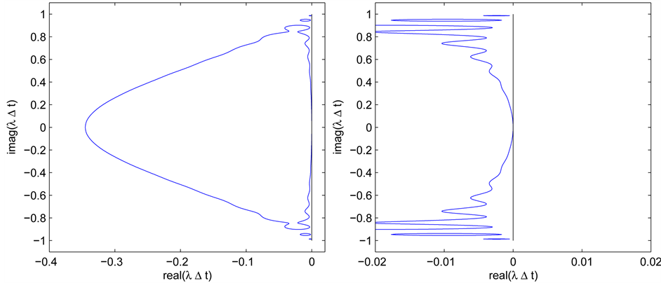
The absolute stability region of the M1 approach with ![]() is shown in Figure 3. In the left image of the figure the stability region is seen to cover significant area in the left half plane and appears to retain coverage of the portion of the imaginary axis over the interval
is shown in Figure 3. In the left image of the figure the stability region is seen to cover significant area in the left half plane and appears to retain coverage of the portion of the imaginary axis over the interval![]() . However, the right image of the figure zooms in on the imaginary axis and reveals that a large portion of the interval is not included in the stability region.
. However, the right image of the figure zooms in on the imaginary axis and reveals that a large portion of the interval is not included in the stability region.
The absolute stability regions of methods M1, M2, M2, and M4 are found in the following manner. For example, the stability region of M1 with ![]() is found by applying the method to the test problem (3). Then the amplification factor
is found by applying the method to the test problem (3). Then the amplification factor ![]() of the method is found by looking at
of the method is found by looking at
![]()
![]()
![]()
![]()
![]()
and
![]()
The absolute stability region contains all the ![]() for which
for which![]() .
.
6.2. Filter, Euler Restart Every N Steps (M2)
Method M2 approximates the first time level with Euler’s method (11) and then advances in time with ![]() leapfrog steps. Then the
leapfrog steps. Then the ![]() filter is applied and the value of
filter is applied and the value of ![]() is assigned to be the filtered average. Then the method is restarted with the initial condition
is assigned to be the filtered average. Then the method is restarted with the initial condition![]() . Thus the method is
. Thus the method is
![]() (45)
(45)
![]() (a) (b)
(a) (b)
Figure 3. (a): Absolute stability region of method M1. (b): close up of the stability region along the imaginary axis.
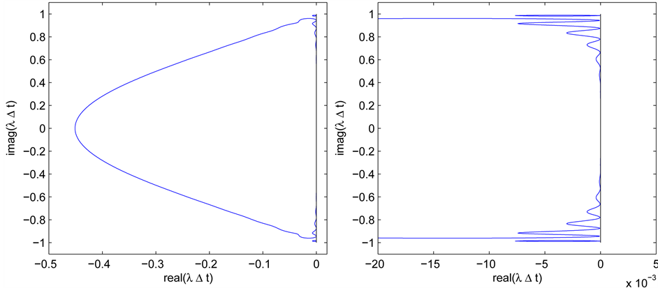
The M2 approach remains second order accurate and requires ![]() function evaluations per time step. In the given example an average of 1.1 function evaluation per time step are needed. The main drawback of approach M2 is that the stability region (Figure 4) lacks any coverage along the imaginary axis. Method M2 is unstable for all values of
function evaluations per time step. In the given example an average of 1.1 function evaluation per time step are needed. The main drawback of approach M2 is that the stability region (Figure 4) lacks any coverage along the imaginary axis. Method M2 is unstable for all values of  for which leapfrog method is absolutely stable.
6.3. Alternative Start/Restart-Algorithm 1 (M3)
The absolute stability region of Euler’s method is a circle of radius one that is centered at  in the complex plane. The region does not include any purely complex numbers. Calculating the first step of method M2 with Euler’s method is causing the method’s stability region to lack imaginary axis coverage.
The following starting procedure
 (46)
(46)
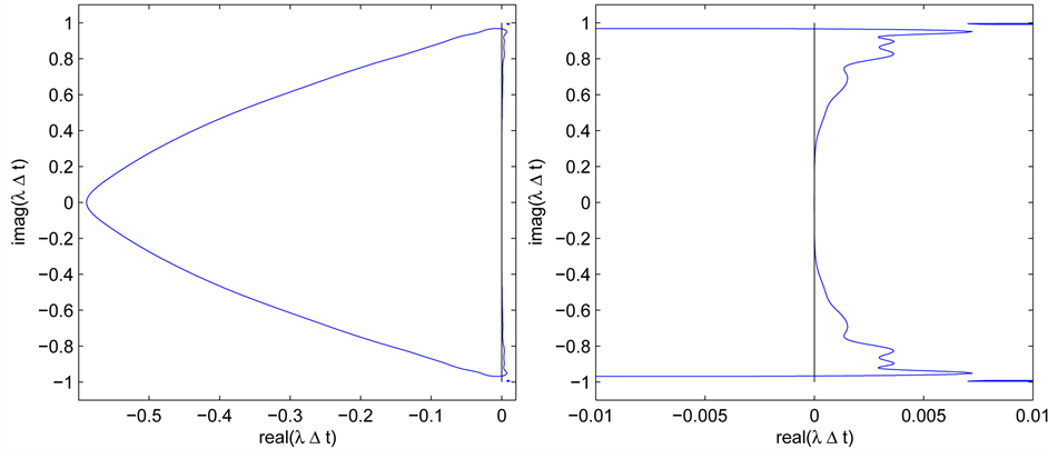
is suggested for minimizing this effect. To advance from the initial condition to time level one, M smaller substeps are taken consisting of one Euler step followed by  leapfrog steps. After the first step, algorithm M3 is identical to algorithm M2. The absolute stability region of method M3 with
  and
and  is shown in Figure 5. The proposed starting procedure has improved the imaginary axis coverage of the stability region to approximately the interval
 , or about half the size of the leapfrog methods stability interval. Method M3 requires
  function evaluations per time step, which in the given example is equal to 1.25. Method M4 in the next section makes one more modification to further increase the coverage of the stability region along the imaginary axis.
6.4. Alternative Start/Restart Algorithm 2 (M4)
Algorithm M4 uses the same starting procedure (46) as does M3 but it does not terminate and restart after filtering at time step N. Instead time levels  and N are filtered and then N more leapfrog steps are taken. The filtering and continuing process is done C times before restarting. At the end of each continuation step the final time level is filtered. The region of absolute stability for the M4 algorithm with
 ,
,  , and
, and  (a total of 21 time steps in order to approximate the 20 time steps used in the M1, M2, and M3 examples) is in Figure 6. The imaginary axis coverage of the M4 stability region is nearly equal to that of the leapfrog method,
 (a) (b)
Figure 4. (a): Absolute stability region of method M2. (b): close up of the stability region along the imaginary axis.
 (a) (b)
Figure 5. (a): Absolute stability region of method M3. (b): close up of the stability region along the imaginary axis.
 (a) (b)
Figure 6. (a): Absolute stability region of method M4. (b): close up of the stability region along the imaginary axis.
covering approximately the interval . The M4 algorithm requires an average of
 function evaluations per time step which is approximately 1.24 in the example given. Matlab source code that implements method M4 is available on the website of the second author at http://www.scottsarra.org/math/math.html.
7. Numerical Results
7.1. Example 1
The purpose of the first example is to demonstrate the ability of the proposed methods to control the computational mode that is introduced by the leapfrog weak instability. The example considers the nonlinear IVP
 (47)
(47)
which has the exact solution . A time step size of
  is used with all methods. Figure 7 illustrated behavior typical of a weakly stable method. Over the finite time interval
  the leapfrog method gives a good approximation to the true solution. Table 3 reports the solution having five digits of accuracy at
 . However, after approximately
 , non-physical oscillations appear in the solution and eventually the solution becomes unbounded.
Table 3 records the results of applying the two new LMMs from section 2 and as well as using the four filter and restart algorithms. Additionally, the five point asymmetric filter  that was recommend in [10] is used. By
  and later, all seven of the filtered method have either zero or near zero error. The numerical solutions nearly exactly approximate the exact solution which becomes the constant
  as
as . In this example, all seven methods have effectively damped the computational mode and prevented the numerical solution from becoming infinite. In five of the methods, graphically non-physical oscillations are not observed. However, in methods
  and M2 slight oscillations (as in Figure 8) appear in the numerical solution prior to the compu- tational mode being damped sufficiently.
7.2. Example 2
This example numerically calculates the order of convergence of the leapfrog method and the seven filtered methods. The test Equation (3) is used with  and with the initial condition
 . Each method is re- peated on the time interval
  using the sequence of number of time steps
 . The resulting convergence plots are shown in the left and right image of Figure 9. On a log-log plot of the absolute value of the error versus the time step size the plot will be a straight line with a slope that is the order of convergence of the method. The LMM3, Asym
  -M2, M1, and
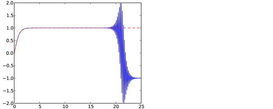
Figure 7. Exact (dashed) and leapfrog (solid) solution of problem (47) with .
.
Table 3. Errors from problem (47).
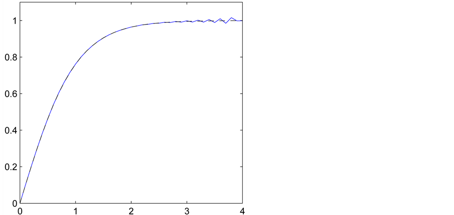
Figure 8. Oscillations appear in the asymmetric  and M2 method solutions prior to the computational mode being damped.
 (a) (b)
Figure 9. Convergence plots. (a): LF, LMM3, LMM5,  -M2. (b): M1, M2, M3, M4. The M3 and M4 plots are visually nearly identical.
M2 methods are only first order accurate while the LMM5, M3, and M4 methods retain the second order accuracy of the leapfrog method. In this example, the three second order accurate filtered methods are about a decimal place more accurate for a given value of k than is the leapfrog method.
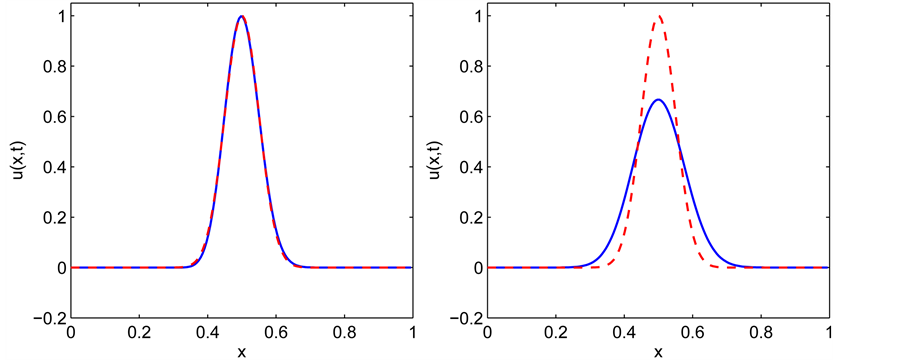
7.3. Advection
The purpose of the third example is to give an illustration of the effects of the dispersion and dissipation properties of the two LMM described in Section 2 and to illustrate the effectiveness of the M4 algorithm as a method of lines integrator of hyperbolic PDEs. A model hyperbolic PDE problem is the advection equation
 (48)
(48)
The domain for the problem is the interval  and periodic boundary conditions are enforced. The initial condition is taken from the exact solution
 .
.
The space derivative of (48) is discretized with the Fourier Pseudospectral method [21] [22] . A relatively large number of points,  , are used to discretize the space interval so that the space errors will be negligible. After discretizing in space the linear system of ODEs
 (49)
(49)
remains to be advanced in time where D is the  Fourier differentiation matrix [23] . The eigenvalues of D are purely imaginary requiring an ODE method with a stability region having imaginary axis coverage. The four methods in this work that are applicable are the leapfrog method, the
  LMM, the
  LMM, and methods M3 and M4. However, the imaginary axis coverage of the stability region of the M3 is small compared to that of M4 so the M3 method is not applied.
Runs with two different time step sizes are made. The first with  and the second with
 , where
  is the magnitude of the largest eigenvalue of D. With the first time step the
  LMM in practically non-dissipative while the second is near the stability limit for the
  LMM. As analyzed in section 6.4, the M4 method is absolutely stable for time step sizes as large as
  for the advection equation. With the maximum stable time step size the error at
  is 3.7e−1. The results at
  are shown in Figure 10 and additional results are in Table 4 and Table 5.
7.4. Advection-Diffusion
Discretized advection-diffusion operators do not have purely imaginary eigenvalues and thus the leapfrog method is not an appropriate method of lines integrator for this type of problem. Advection-diffusion problems in which the advection term is dominant will have differentiation matrices with eigenvalues that have negative real parts that are of small to moderate size. Algorithm M4 can be effectively applied in such a problem.
 (a) (b)
Figure 10. Solutions of problem (48) at  (exact dashed, numerical solid) with
 : (a):
  LMM; (b):
  LMM.
LMM.
Table 4. Errors from problem (48), .
.
As an example, the advection diffusion equation
 (50)
(50)
where  is considered. The viscosity coefficient is taken as
  and periodic boundary conditions are applied on the interval interval
 . The space derivatives are discretized with the Fourier Pseudospectral method with 199 evenly spaced points. The scaled spectrum of the discretized space derivative operators and the stability region of method M4 is shown in the left image of Figure 11. An initial condition of

is used and the problem is advanced in time to  using a time step of
 , where
  is the maximum magnitude of the imaginary part of the eigenvalues of the discretized operator. In the right image of Figure 11 the numerical solution at
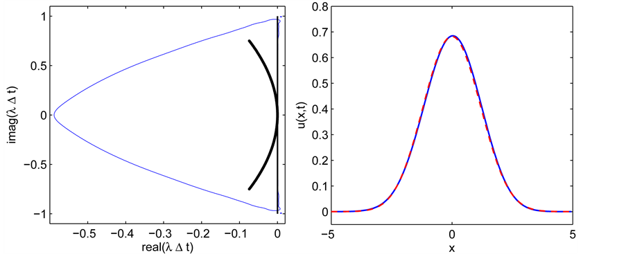
  is compared with the exact solution. The maximum error is 1.3e−2. The results illustrate the ability of method M4 to accurately advance advection dominated problems over long time intervals.
8. Conclusion
Filters of length three and five have been examined for the purpose of controlling the weak instability of the leapfrog method. Filtering the leapfrog method with a three point filter reduces the accuracy of the overall scheme to first order. If a five point filter is used, it is possible for the method to retain the second order accuracy as well as damp the computational mode by a factor of . Several ways of incorporating the filter into the leapfrog method have been examined. Applying the five-point symmetric filter to the time level
Table 5. Errors from problem (48), .
.
 (a) (b)
Figure 11. (a): Stability region of method M4 and the scaled spectrum of the discretized problem (50); (b): Numerical solution (solid) vs. exact (dashed) at .
.
of the leapfrog method (9) results in a new second order accurate LMM (43) which is zero stable and that has an absolute stability region that includes both coverage of a portion of the imaginary axis as well as a region in the left half plane. Of the four filter and restart algorithms described, algorithm M4 is the most attractive. The M4 method, which restarts after every 21 time steps, has an absolute stability region that includes nearly as much of the imaginary axis as does the leapfrog method as well as includes a region in the left half plane. This allows the method to be an effective method of lines integrator for pure advection and advection dominated problems as is illustrated in the examples. In addition to the second order accuracy, the method also retains the computational efficiency of the leapfrog method. Method M4 is a potential replacement for existing leapfrog type time differencing schemes that are used in geophysical fluid dynamics codes.
Cite this paper
Ari Aluthge,Scott A. Sarra,Roger Estep, (2016) Filtered Leapfrog Time Integration with Enhanced Stability Properties. Journal of Applied Mathematics and Physics,04,1354-1370. doi: 10.4236/jamp.2016.47145
References
- 1. Richardson, L.F. (1922) Weather Prediction by Numerical Process. Cambridge University Press, Cambridge.
- 2. Williams, P. (2009) A Proposed Modification to the Robert-Asselin Time Filter. Monthly Weather Review, 137, 2538-2546.
http://dx.doi.org/10.1175/2009MWR2724.1 - 3. Coiffier, J. (2011) Fundamentals of Numerical Weather Prediction. Cambridge University Press, Cam-bridge.
http://dx.doi.org/10.1017/CBO9780511734458 - 4. Butcher, J. (2003) Numerical Methods for Ordinary Differential Equations. Wiley.
http://dx.doi.org/10.1002/0470868279 - 5. Milne, W. and Reynolds, R. (1959) Stability of a Numerical Solutions of Differential Equations. Journal of the ACM, 6, 196-203.
http://dx.doi.org/10.1145/320964.320976 - 6. Asselin, R. (1972) Frequency Filter for Time Integrations. Monthly Weather Review, 100, 487-490.
http://dx.doi.org/10.1175/1520-0493(1972)100<0487:FFFTI>2.3.CO;2 - 7. Gragg, W.B. (1963) Re-peated Extrapolation to the Limit in the Numerical Solution of Ordinary Differential Equations. PhD Thesis, UCLA.
- 8. Bulirsch, R. and Stoer, J. (1966) Numerical Treatment of Ordinary Differential Equations by Extrapolation Methods. Numerische Mathematik, 8, 1-13.
http://dx.doi.org/10.1007/BF02165234 - 9. Shampine, L. and Baca, L. (1983) Smoothing the Extrapolated Midpoint Rule. Numerische Mathematik, 41, 165-175.
- 10. Iri, M. (1963) A Stabilizing Device for Unstable Numerical Solutions of Ordinary Differential Equations—Design Principle and Application of a Filter. Journal of the Information Processing Society of Japan, 4, 249-260.
- 11. Li, Y. and Trenchea, C. (2014) A Higher-Order Robert-Asselin Type Time Filter. Journal of Computational Physics, 259, 23-32.
http://dx.doi.org/10.1016/j.jcp.2013.11.022 - 12. Norton, T. and Hill, A. (2015) An Iterative Starting Method to Control Parasitism for the Leapfrog Method. Applied Numerical Mathematics, 87, 145-156.
http://dx.doi.org/10.1016/j.apnum.2014.09.005 - 13. Dahlquist, G. (1985) 33 Years of Numerical Instability, Part I. BIT, 188-204.
http://dx.doi.org/10.1007/BF01934997 - 14. Todd, J. (1950) Solution of Differential Equations by Recurrence Relations. Mathematical Tables and Other Aids to Computation, 4, 39-44.
http://dx.doi.org/10.2307/2002701 - 15. Hairer, E., Norsett, S. and Wanner, G. (2000) Solving Ordinary Differential Equations I: Nonstiff Problems. Springer.
- 16. Hairer, E. and Wanner, G. (2000) Solving Ordinary Differential Equations II: Stiff and Differential—Algebraic Problems. 2nd Edition, Springer.
- 17. Henrici, P. (1962) Discrete Variable Methods in Ordinary Differential Equations. Wiley.
- 18. Iserles, A. (1973) A First Course in the Analysis of Differential Equations. Wiley.
- 19. Lambert, J. (1973) Computational Methods in Ordinary Differential Equations. Wiley.
- 20. Aluthge, A. (1985) Filtering and Extrapolation Techniques in the Numerical Solution of Ordinary Differential Equations. Master’s Thesis, University of Ottawa, Ottawa.
- 21. Boyd, J.P. (2000) Chebyshev and Fourier Spectral Methods. 2nd Edition, Dover Publications, Inc., New York.
- 22. Canuto, C., Hussaini, M., Quarteroni, A. and Zang, T. (1988) Spectral Methods in Fluid Dynamics. Springer.
http://dx.doi.org/10.1007/978-3-642-84108-8 - 23. Weideman, J.A.C. and Reddy, S. (2000) A MATLAB Differentiation Matrix Suite. ACM Transactions on Mathematical Software, 26, 465-519.
http://dx.doi.org/10.1145/365723.365727