Theoretical Economics Letters
Vol.4 No.6(2014), Article
ID:46841,15
pages
DOI:10.4236/tel.2014.46055
Socially-Optimal Locations of Duopoly Firms with Non-Uniform Consumer Densities
Kieron J. Meagher1, Ernie G. S. Teo2, Taojun Xie3
1Research School of Economics, Australian National University, Canberra, Australia
2Sim Kee Boon Institute of Financial Economics, Singapore Management University, Singapore
3Division of Economics, Nanyang Technological University, Singapore
Email: kieron.meagher@anu.edu.au, ernieteo@smu.edu.sg, txie1@e.ntu.edu.sg
Copyright © 2014 by authors and Scientific Research Publishing Inc.
This work is licensed under the Creative Commons Attribution International License (CC BY).
http://creativecommons.org/licenses/by/4.0/


Received 11 April 2014; revised 11 May 2014; accepted 2 June 2014
Abstract
Advances in the theoretical literature have extended the Hotelling model of spatial competition from a uniform distribution of consumers to the family of log-concave distributions. While a closed form has been found for the equilibrium locations for symmetric log-concave distributions, the literature contains no closed form solution for the socially optimal locations. We provide a closed form solution for the socially optimal locations: one mean-deviation away from the median. We also derive a formula for the excess differentiation ratio which complements the bounds previously derived in the literature, and establish the invariance of this ratio to a form of mean preserving spread. The equilibrium duopoly locations of several types of commonly used distributions were discussed in [1] . This paper provides the closed form solutions for the socially optimal locations to the same set of distributions. We calculate welfare improvements arising from regulation of firm location and show how these vary with the distribution of consumers. While regulating firm locations is sufficient to optimize welfare for symmetric distributions, additional price regulation is required to ensure social optimality for asymmetric distributions. These results are significant for urban policy over firm/store locations.
Keywords
Socially Optimal Firm Locations, Distributions, Spatial Competition, Duopoly

1. Introduction
Transport costs are a primary driver of the location decisions of firms in models of spatial economics. Transport costs can occur in an enormous range of contexts: inputs costs for intermediate products or in commute times for workers; or in output markets as search costs, shopping costs or delivery costs for consumers. A large, but by no means exhaustive, survey is provided by [2] . From a firm’s perspective the essential issue of spatial economics is that it cannot be close to everything1. Identifying how firms handle this trade-off in choosing locations, and how these choices impact on society, gives rise to a central research theme of the literature, and it is to this area that this paper contributes.
Most theoretical firm location models assume a uniform consumer distribution; this is seldom observed in real life. In their seminal contributions [3] and [4] established the existence of price equilibrium for log-concave densities. [5] extended this line of research by providing sufficient conditions for the existence of pure strategy location-price equilibrium for log-concave consumer densities, and for the symmetric case, a closed form equation for the equilibrium locations and prices.
The analysis of socially optimal locations in the literature has not established a closed form for the socially optimal locations and as a result the comparison of equilibrium and optimal locations—in terms of the ratio of competitive product differentiation to the optimal differentiation—has produced bounds but not an exact result. We fill this gap by providing explicit formulas for both the socially optimal locations and the ratio of equilibrium to optimal differentiation.
The research questions of this paper are: 1) what are the socially optimal locations of firms within the canonical, quadratic Hotelling model; and 2) how do the equilibrium, firm level location decisions compare with the socially optimal locations? Our contribution is to extend the analysis of social optimality beyond the typical assumption of uniformly distributed consumers. In most real world settings, non-uniform consumer distributions would be more realistic—our results apply to important specific densities like the Normal and Logistic. One of the few theoretical works, which utilizes a non-uniform consumer distribution, is that of [6] where a symmetric triangular density was used. This is extended in unpublished work by [7] , where the consumer distribution can take several forms ranging from uniform (rectangular) to triangular (densities in-between the two assume a trapezoidal shape). In [8] , a state space approach where different states give rise to different consumer distributions was used to model uncertainty in spatial duopolies.
[1] identified a list of distributions where unique pure strategy equilibrium exists and also determines their locations. This paper follows [1] and examines the socially optimal locations of these distributions. Although [9] showed that there is excessive differentiation in the uniform case of the two-stage location-price game, and [5] supports the existence of excessive differentiation by deriving bounds results about the social-optimum locations; we are the first to examine precisely excess differentiation for a wider range of specific distributions, including asymmetric distributions.
The amount of differentiation and the total transport cost2 savings from government intervention are discussed in this paper. We also consider the effect of regulating the firms to the social-optimum locations and allowing them to set competitive prices. This decomposes the welfare gains from regulation into spatial and pricing decisions. This separation is important in practice because location in many industries is much cheaper to regulate/monitor than prices.
Using location as a form of regulation is of interest to governments. For example, the Australian Competition and Consumer Commission found in an inquiry into grocery stores in Australia that incumbent supermarkets have used planning objection processes to deter new entry thus lessening competition. Proceedings in the UK Competition Commission inquiry into Groceries [12] resulted in legal orders regulating the location related behavior of large grocery chains. Governments may use location regulation as a means to regulate competition.
Pricing regulation is hard to administer when stores sell a variety of products. The Australian government attempted to regulate prices of grocery chains by publishing the prices charged by each store for a basket of goods; this proved to be too costly and the website was shut down [13] . This may indicate that location regulation may be a more feasible way to ensure social welfare.
The question of price regulation is only binding under asymmetry, and hence prior to our analysis of asymmetric densities, price regulation could not be considered in any meaningful way3. There is of course more to the location of a firm than the stylized Hotelling model, but it is the workhorse of spatial competition and as we show the welfare implications are sensitive to the choice of consumer distribution.
2. Social-Optimum Location in the Quadratic Transport Cost Model
We use a quadratic transport cost model as specified in [9] , but generalize beyond uniform consumer density. There are two firms on the real line and each produces a homogeneous good at a constant marginal cost, henceforth normalized to zero. Firm i is located at xi, where I = 1, 2. Without loss of generality, the firm on the left will be denoted as firm 1 and the firm on the right will be firm 2, x1 ≤ x2. There is a continuum of consumers, whose mass is normalized to unity without loss of generality. The transport cost incurred by the consumer located at x from consuming the good at xi is:
 (1)
(1)
where t is the amount it costs to travel to purchase the good. For simplification, we let t = 1.
The consumer density is , ≥for all x, and its cumulative distribution function is denoted by
 . We assume
  is twice differentiable on its support [a, b], where a may be −∞ and/or b can be ∞.
The social-optimum problem is simply to minimize the aggregate transport costs, T, in serving consumers:
 (2)
(2)
where µ is the boundary between the group of consumers who go to firm 1 and those who go to firm 2. Since demand is inelastic and production costs are constant and identical across firms, the socially optimal value of µ, denoted µs, is
 . (3)
. (3)
since it is clearly optimal to serve each consumer from the closer firm.
Remark 1. As shown in [5] , if  is logconcave then the first order conditions yields the unique socially optimal locations, i.e. the unique solution to the programme
 (4)
(4)
2.1. Logconcave Consumer Densities
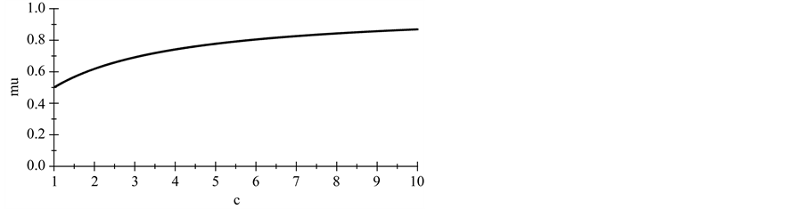
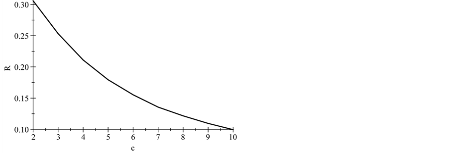
Given Remark 1, we naturally restrict attention in this paper to logconcave densities. Although logconcavity is sufficient for the existence of a unique pair of socially optimal location, additional conditions are required to guarantee existence of a unique competitive equilibrium, see [5] . Table 1 contains the list of distributions proven in [1] to satisfy the conditions for the existence of unique location-price equilibria. 2.2. Social-Optimum Locations A generic set of implicit conditions for the social-optimum locations, in terms of integral equations, is given in [5] . The pair of social-optimum locations (which minimizes and where µS solves Table 1. Standardized forms of the consumer densities considered. Building on these results, we provide an explicit characterization of the socially optimal locations for symmetric distributions. Proposition 1. For any symmetric, log-concave distribution with a mean/median of M and mean-deviation Proof. Let To prove the proposition, we need to show that this distance equals one mean deviation or Since X is symmetrically distributed, on the left-hand-side, Integrating by parts gives and on the right-hand-side, which establishes the result for M = 0. Extension to M ≠ 0 is trivial. ■ For log-concave densities, symmetry of the density is sufficient to make the socially optimal locations of the two firms symmetric about the median/mean of the consumer density. One might expect that as consumer locations become more dispersed, the locations of the two firms should also become further apart. We show in Proposition 3 on spread that this loose intuition is precisely true to the degree that dispersion of consumer preferences is measured by the mean deviation. With a formula for the socially optimal locations in hand, it is now possible to analyze the excess differentiation of the competitive locations compared to the socially optimal locations. Using results from Proposition 1, we solve the system of equations4 for each of the density functions which satisfy [5] ’s three conditions (i.e. the distributions listed in Table 1)—the results are given in Proposition 2. Proposition 2. The socially optimal locations and transport costs for five of the logconcave distributions given in Table 2, where Proof. See online working paper at: http://dx.doi.org/10.2139/ssrn.1615884. ■ The results for the Uniform case are already well known; the results for the other four distributions are new and allow for an analysis of spatial competition in the Hotelling framework which is no longer tied to the uniform distribution. The Rayleigh distribution is asymmetric and has socially optimal locations which are not symmetric about either its mean (≈0.886) or its median (≈0.833). Thus the symmetry result for the first four distributions in Proposition 1 does not hold in general for asymmetric densities. In the Rayleigh case the left firm is located in the dense left part of the distribution and the right firm is located well out into the long right tail which goes off to infinity. The locations are sufficiently to the right to place the boundary µS to the right of the median and the mean. Table 2 shows that the optimal differentiation between the two firms varies considerably with the shape of the consumer density function and therefore the choice of density utilized in analyzing the Hotelling model could have a significant impact on the results. We benchmark the impact of the distribution shape below in two ways. First, in Section 3, we compare the socially optimal locations with the competitive equilibrium locations and find how savings on transportation costs varies across distributions. Second, in Section 4, we go beyond the standardized functional forms above to compare the social optimum results for different distributions as the dispersion of the distributions increases. The “standardized” versions of the Power and Weibull distributions depend on the parameter c, and as a result the socially optimal locations also depend on c. The more involved results for these two families are presented in the next section. 2.3. Special Cases: Asymmetric Distribution Next, we look at the social optimum locations of two asymmetric families of distributions, specifically, the Weibull and the Power distributions. 2.3.1. The Weibull Distribution The Weibull distribution has no explicit solution for µS. In this section, we look at the solution to the Weibull distribution in detail. µS for the Weibull distribution solves the following equation: Equation (Weibull) involves the integral of 2.3.2. The Power Distribution Similarly, there is no explicit solution for the Power distribution either. Here, we find µS that solves the integral equation for the Power distribution: Table 2. Social-optimum locations for density functions which satisfy the conditions in [5] . The above can only be solved explicitly for fixed levels of c. Hence the value of µS depends on c. To examine the relationship between µS and c, the following total differential equation is obtained. The first part on the right-hand-side, Knowing the direction of change of µS resulted from a change in c, we can now derive the change in A check on the second order conditions for dµS/dc shows that it is a concave function with maximum value at µS = 0.5 and c = 1, i.e. since the denominator increases at a faster rate than the numerator. From here we know that the deviation of firms’ locations from µS decreases as µS approaches 1. As such, product differentiation decreases as the curvature of the density function increases. To illustrate, we plot the graph of µS against c and solve numerically for Power distributions with integer values 2 ≤ c ≤ 10. The graph and values are in Figure 1 and Table 3 respectively. It can be observed that µS is increasing in c and the two socially optimum locations get closer as c increases. However the increase of the market boundary for firm 1 does not translate in to an increase in market share for firm 1 because the density is also changing shape in c. For example, at c = 2, firm 1 serves 38.2% of the market while at c = 10 firm 1’s market share falls to 24.5%. The amount of differentiation will be discussed in detail in the next section. 3. Equilibrium and Social-Optimum Differentiation [1] derive the bounds for the ratio between social-optimum and equilibrium differentiation for symmetric distributions. Specifically they find Table 3. The social-optimal locations under the Power distribution. Figure 1. Graph of µS against c. where R is inversely proportional to the amount of excess differentiation. These bounds show there is always substantial excess differentiation in the location-price game [5]
 ) are the
  that solve:
 (5)
(5) (6)
(6) (7)
(7) , the social-optimum duopoly locations are one mean-deviation away from the median:
 (8)
(8) be a symmetric, log-concave probability density function with supports (−b, b) and median M = 0. [5] have shown that the socially optimal locations for duopoly firms are symmetric around the median for distribution
 . The distance between either firms and the median is
 (9)
(9) (10)
(10) (11)
(11) (12)
(12) (13)
(13) ’s are the social-optimum location for firm i, and TS’s are the social-optimum transportation costs.
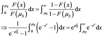 (14)
(14) of which the closed form cannot be determined for c > 2. The Exponential and the Rayleigh distributions are the Weibull with c = 1 and c = 1 respectively. For the exponential distribution, we find that
 ,
,  and µS = 1.5936. However, as proven in [1] , the Exponential distribution does not satisfy the conditions for the existence of unique location-price equilibria. Thus, for the class of Weibull distributions, only the Rayleigh distribution will be discussed in the subsequent sections. For the Rayleigh distribution, we find that µS = 0.97213, and the social-optimum locations are
 ,
, .
. (15)
(15) (16)
(16) , is positive. To determine the sign of the second part, we check the first order conditions and concavity of the numerator and denominator. The result shows that both functions are positive given the constraints c ≥ 1,
  and Equation (15) holds. Therefore, the value of µS increases with c, where c determines the curvature of Power distribution’s density function.
 and
and  from Equations (5) and (6). The deviation of firms’ location from µS is
 (17)
(17) . We then have
 (18)
(18)
 (19)
(19) (20)
(20)
Proposition 3. If consumers are distributed according to a continuous, log-concave, symmetric density f on  which satisfies the technical restrictions of [5] 6 then
 (21)
(21)
and the differentiation ratio,  , is invariant to the mean preserving spreads of the form
 , with s > 0, i.e.
 .
.
Proof. From [5] , the conditions on f give . The expression for R then follows from direct substitution of the previous proposition:
 (22)
(22)
Using this explicit expression we now derive the invariance result, without loss of generality assume M = 0. Let Es denote the expectation with regard to the distribution fs, then
 (23)
(23)
where z = y/s. Simple substitution gives the result with M ≠ 0. Thus for the mean preserving spread given by fs we have
 (24)
(24)
For this type of mean preserving spread, the increase in the absolute deviation from the median/mean is linear in s while the decrease in the density of the mean is at the rate 1/s, so the two effects exactly balance. That is, in this case the tendency for socially optimal locations to increase because of greater dispersion is proportionally the same as the tendency for competitive locations to move apart due to decreased competition for the marginal consumer at M.
The exact amount of differentiation that each distribution results in is shown in Table 4 and Table 5. As [5] observe that amongst the symmetric distributions the Uniform and Laplace distributions exhibit the greatest and least divergence respectively. However, in extending the analysis to asymmetric distributions, we see that asymmetric distributions have greater divergence than any of the symmetric distributions in the group.
For the Power distribution, under a duopoly location-then-price game, the product differentiation7 is
 (25)
(25)
The first derivative is
 (26)
(26)
so the amount of product differentiation increases as c increases. Examples are given in Table 5. Since the product differentiation increases under equilibrium and decreases under social-optimum conditions, the amount
Table 4. Amount of differentiation (x2 − x1) for equilibrium and social-optimum locations and their ratios.


 , firms maximize profits by setting prices at:
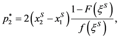
 . Hence,
 . This requires both firms to charge equal price, i.e. p1 = p2. We check if the location combination
  support equal price for each of the distributions mentioned previously. For any given symmetric density function, the prices of the two firms will be equal8. This is not true for asymmetric distributions, such as the Power and Rayleigh distributions.


 . Equation (35) contradicts our assumption that X has an asymmetric density function. As such, M is not a solution to Equation (7). ■


 , and hence x = M. In addition, substituting x = M into Equation (38), we have
 . Therefore, the locations of the two firms are symmetric about the indifferent consumer when the prices are equal. ■
 and competitive prices. By Lemma 1, the median M is not a solution (for asymmetric distributions) to Equation (7), i.e. M ≠ µS. The social-optimum locations are symmetric about µS as implied by Equations (5), (6) and (7). Hence these social-optimum locations are not symmetric about the median M. Taking the contrapositive of Lemma 2 implies that firms’ competitive prices are not identical at the socially optimal locations. Next, we show that this set of locations with non-equal prices are not welfare maximizing.
 . Suppose xS > µS, consumers located at the interval (µS, xS) would pay a higher transportation cost to buy goods from firm 1 while it incurs less cost to buy the same goods from firm 2. On the other hand, if xS < µS, buying goods from firm 2 would incur higher transportation cost for consumers in the interval (xS, µS). The transportation costs spent by consumers in the interval (min(xS, µS), max(xS, µS)) are not minimized while that spent by all the other consumers are. We then arrive at the conclusion that the society’s transportation costs are higher when xS is different from µS. Thus, we have shown that the sole regulation of locations do not eventually result in transportation cost minimization. What happens if prices are regulated too?
 . Equations (36) and (37) can be disregarded as firms do not have the freedom to set the prices. According to Equation (31), the indifferent consumer, xS, is now located at
 , which is exactly the location of µS. All consumers would then buy goods from whichever firm that is closer to them. The society’s total transportation cost is minimized as each single consumer’s transportation cost is minimized. That completes the proof of the proposition. ■
 and
and . The results are listed in
  this denotes the savings in transport costs as a result of switching from the equilibrium locations to the social-optimal. In
  , xS > µS. This means consumers located at the interval (µS, xS) would buy goods from firm 1 while it incurs less transportation cost to buy from firm 2. Therefore, the society’s costs are not minimized in this case.
 and
and . The resulting indifferent consumer is at x = 0.8787, which is on the left of µS. Consumers located at 0.8787 < x < 0.9721 would buy goods from firm 2 while it incurs less transportation cost to buy from firm 1. The transportation costs for consumers in this interval are not minimized, and hence society’s total transportation cost is not the minimum. The saving ratio (S) for the Rayleigh distribution is 0.900 and is smaller than when the firms are forced to set equal prices where S = 0.907.