Theoretical Economics Letters
Vol.4 No.3(2014), Article ID:44923,6 pages DOI:10.4236/tel.2014.43032
Valuing Carbon Recycling through Ethanol: Zero Prices for Environmental Goods
Charles B. Moss, Andrew Schmitz
University of Florida, Gainesville, USA
Email: aschmitz@ufl.edu, cbmoss@ufl.edu
Copyright © 2014 by authors and Scientific Research Publishing Inc.
This work is licensed under the Creative Commons Attribution International License (CC BY).
http://creativecommons.org/licenses/by/4.0/


Received 17 January 2014; revised 17 February 2014; accepted 7 March 2014
ABSTRACT
The Energy Independence and Security Act of 2007 imposes a Renewable Fuel Standard met through a combination of corn and cellulosic ethanol. A variety of rationales support this policy including the recycling of atmospheric carbon. This study examines the economic dimensions of this problem focusing on the role of zero prices for environmental goods and the use of an environmental equivalent. When environmental goods are taken into account, the optimal price policy cannot be defined with certainty.
Keywords:Ethanol, Renewable Fuel Standard, Volumetric Ethanol Excise Tax Credit, Market Failure

1. Introduction
The Renewable Fuel Standards (RFS) introduced in the Energy Independence and Security Act of 2007 draws support from a wide array of policy goals. Among the most prominent are the support the RFS provides for agricultural prices largely through the increased demand for corn and the potential environmental benefits of biofuels. The later includes the possible effect of carbon recycling. Specifically, the production of ethanol implies that carbon removed from the atmosphere can be used to replace incremental carbon that would be produced from oil. This contention has been the subject of significant debate in the guise of the carbon cycle [1] . However, the economic impacts of these potential environmental effects can be developed within the context of a general equilibrium model.
The value of removing atmospheric carbon is problematic (that is true with many environmental goods) since no market price exists for this environmental amenity since it is not traded in an identified market. One view is that a zero price for the environmental good implies that it is in equilibrium if the excess supply of the environmental good is less than zero, or the supply of the environmental amenity exceeds the demand. The contrasting view is that the typical market demand for these environmental goods exceeds the observed market demand for a variety of reasons (i.e., the free-rider problem where consumption is nonexclusionary). Hence, the existing zero price for these environmental goods understates their scarcity in the economy. In case of biofuels, the zero value of the reduction in atmospheric carbon could imply market failure. Under the RFS, this market failure could be reduced by including a value for atmospheric carbon (i.e., the Volumetric Ethanol Excise Tax Credit [VEETC] which expired in 2012 provided a mechanism to correct such a market failure). This study develops this tradeoff within the context of a general equilibrium model. In addition, we discuss the implications of market failure using the concept of an environmental equivalent (the amount of benefit that the economy must receive from an environmental policy to yield a benefit cost ratio of one) introduced by Schmitz, Kennedy, and Hill Gabriel [2] .
2. Standard Formulation of the General Equilibrium
Consider the standard formulation of the applied general equilibrium model where there exists a numerical set of prices  (where
  is the price of outputs or consumables and
  is the price of the household’s endowments or factors of production) can be found such that all the excess demand relationships
 (1)
(1)
where  is the consumer’s demand for good
 ,
,  is the supply curves for each good, and
  is the demand for the factors of production
 .
.
Applied work models such as GEMPACK [3] and GTAP [4] expand the formulation to allow for intermediate outputs. Specifically, as depicted in Figure 1, some of the factors of production are used to produce intermediate products that are then used by other firms to produce final outputs. In this configuration, the factor endowments  are used to produce intermediate inputs
 . The production of consumption goods are then a function of these intermediate inputs and factor endowments. To develop the model further we assume that producers of intermediate inputs maximize profits based on levels of intermediate factors of production
 (2)
(2)
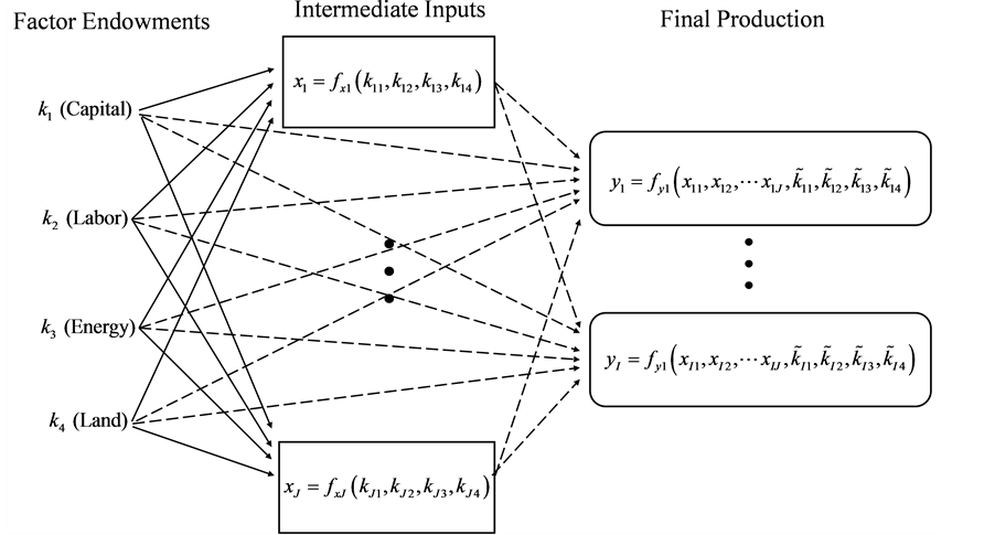
Figure 1. Extended general equilibrium formulation.
where  is the price of intermediate product
 ,
,  is the vector of factor endowment prices,
  is the technology set for the production of product
 ,
,  is the quantity of intermediate input
  supplied for any set of input and output prices, and
  is the input demand for factor of endowment
 . The production of final products or consumption items are then determined by the profit maximization problem
 (3)
(3)
where  is the output price for output
 ,
,  is the vector of intermediate input prices,
  is the level of factor endowment
  used in the production of output
  (as opposed to the use of the same input to produce intermediate outputs), the vector of these choices is denoted
 ,
,  is the technology set for the production of output
 , and
, and  is the level of consumption good
  supplied for a given set of input and output prices.
The results in Equations (2) and (3) provide a slightly more expansive set of general equilibrium conditions
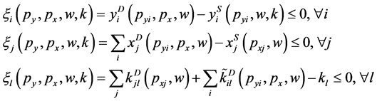 . (4)
. (4)
Expanding the conditions in Equation (4) yields
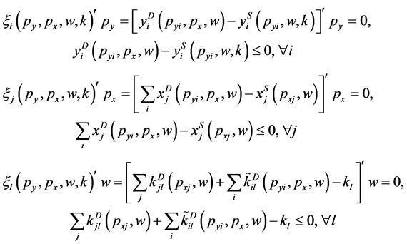 (5)
(5)
incorporating the complementary slackness conditions (i.e., negative excess demands imply non-positive prices).
3. Zero Prices and Environmental Goods
Consider both consumption and production uses of environmental goods. We build on the complementary slackness conditions in Equation (5) by dividing the set of all resource endowments into two groups  such that
  and
and  such that
 . Thus, group
  are priced factors of production while
  are unpriced factors of production. If we ignore the degeneracies (i.e., those points where both the price and the excess demand are both zero), the general equilibrium solution implies that
 (6)
(6)
or in the general equilibrium solution the economy has more of a particular factor endowment than required to maximize society’s utility. The typical goods cited as an example of Equation (6) are sunlight, seawater, or possibly atmospheric nitrogen. These factor endowments do not constrain production. However, it is possible that some of the zero priced goods do not fall in this category because of consumption market failures where non-negative excess demand exists at a zero price.
To develop this concept more completely, consider a slight modification to Equation (6)
 (7)
(7)
where  denotes the demand for a consumption good associated with a factor endowment (i.e., clean air or water, or possibly carbon recycling). Thus, a general equilibrium solution would require a negative excess demand in Equation (7) given that the associated price is equal to zero–or that the price of the environmental endowment equals zero. The concept behind the failure of environmental markets is that
  denotes the market demand for environmental characteristics. However, because of market failures the true demand for the environmental good lies to the right of the market demand curve
 (8)
(8)
where  is the true demand curve. As depicted in Figure 2, the observed market equilibrium for factor
  implies that
 ; however, if we use the “correct” consumer demand curve for the environmental amenity the market price should be
 . At this market price less of the factor endowment will be used in the production of other goods and services
 . (9)
. (9)
The argument is that moving to the solution in Equation (9) improves societal welfare, but this move is not necessarily Pareto improving–there may be gainers and losers.
The critical point is that the size of the error in the observed demand is completely unobserved. For example, if we could observe , the implied error would be
 . (10)
Hence, as long as  the optimal price level for the environmental amenity is still zero. The real problem with the analysis is that one only observes
 . Economic data are not collected on the derived demand for the production of other goods, or even the level of consumption ofdemand specified by the consumer demand curve
 , let alone the true demand curve for the environmental factor.
Figure 3 presents the implications of imposing an ad hoc price (i.e., tax) on the environmental good. The ob-
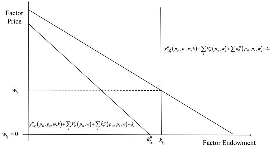
Figure 2. Implicit factor market.
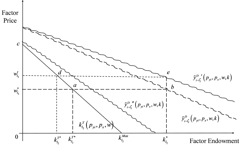
Figure 3. Valuing the environmental equivalent.
servable component of this demand can be measured by the derived demand for the environmental good used to produce other inputs and outputs
 . (11)
Consider three possible consumer demand curves for the environmental variable.
Ÿ Following Equation 8, we define  as the demand curve that justifies the efficient price
 for the environmental good. The corresponding environmental equivalent is
  that represents the value society must place on this environmental good for the cost/benefit ratio of the tax to equal 1.0 (Schmitz, Kennedy, and Hill-Gabriel, 2012). Businesses pay a total tax of
  and earn a surplus from the use of the resource of
 . Note that these costs and benefits are spread across all the outputs that use this environmental good as an input.
Ÿ Next, consider where the consumer value of the environmental good shifts rightward to  (where the squiggled lines are used to denote uncertainty in the exact position of these demand curves). Under this scenario the optimal price of the environmental good increases to
  hence the environmental equivalence increases to
  while the amount tax paid by producers becomes
  (note that the change
  could either be negative or positive depending on the elasticity of the de rived demand curves).
Ÿ Finally there is the case where the value of the environmental good to consumers is . The appropriate price of the environmental good and the value of environmental equivalents are both zero. In that case,
  of the environmental good is used as an input to other production processes and the value of this use is
 .
.
Given these three scenarios, we hypothesize three consequences of setting the price of the environmental good at . In the first scenario, policy makers appropriately value environmental goods. Society realizes an environmental value of
 , producers earn a surplus of
 , and the government collects a tax of
 . If the true demand for the environmental good is
 , pricing the environmental good at
  implies a loss as measured by the environmental equivalent of
  and a change in producer’s surplus from the derived demand for the environmental input of
 . If the derived demand is price inelastic, this change is positive. However, if the derived demand is price elastic this change in producer surplus is negative. Finally, if the true demand for the environmental good is
  the true value of environmental equivalent is zero and imposing a price of
  on the environmental good costs the economy
  which is distributed across all goods produced and consumed in the economy.
4. Conclusion
Placing a value on environmental goods will be a subject of debate for quite some time. This is part of the reason why there is so much controversy surrounding the biofuels mandate. If there are large benefits derived from an environmental perspective, the net gains to policies such as the Volumetric Ethanol Excise Tax Credit can be positive. However, proving amenities exist is problematic. In addition, a whole host of factors play a role in determining the goodness of these type of policies including the effect of policy instruments on other markets that can only be developed in a general equilibrium context [5] [6] .
References
- Babcock, B.A., Rubin, O. and Feng, H. (2007) Is Corn Ethanol a Low-Carbon Fuel? Iowa Ag Review Online, 13. http://www.card.iastate.edu/iowa_ag_review/fall_07/article1.aspx.
- Schmitz, A., Kennedy, P.L. and Hill-Gabriel. J. (2012) Restoring the Florida Everglades through a Sugar Land Buyout: Benefits, Costs, and Legal Challenges. Environmental Economics, 3, 74-85.
- Harrison, J., Horridge, M., Jerie, M. and Pearson, K. (2013) GEMPACK Manual. Monash University, Melbourne. http://www.monash.edu.au/policy/gpdoc.htm
- Hertel, T.W. (1997) Global Trade Analysis: Modeling and Applications, Cambridge University Press, Cambridge.
- Moss, C.B. and Schmitz, T.G. (2011) The Potential Effect of Ethanol on the U.S. Economy: A General Equilibrium Approach. In: Schmitz, A., Wilson, N., Moss, C. and Zilberman, D., Eds., The Economics of Alternative Energy Sources and Globalization, Bentham eBooks, Oak Park, Illinois, 35-49.
- Schmitz, A., Moss, C.B. and Schmitz, T.G. (2007) Ethanol: No Free Lunch. Journal of Agricultural & Food Industrial Organization, 2, Article 3. http://www.bepress.com/jafio/vol5/iss2/art3