Theoretical Economics Letters
Vol. 3 No. 1 (2013) , Article ID: 28164 , 13 pages DOI:10.4236/tel.2013.31009
Mixed Strategy Nash Equilibria in Signaling Games
1Department of Economics and Business, Virginia Military Institute, Lexington, USA
2Department of Mathematics and Computer Science, Virginia Military Institute, Lexington, USA
Email: *cobbbr@vmi.edu, basuchoudharya@vmi.edu, hartmangn@vmi.edu
Received December 3, 2012; revised January 5, 2013; accepted February 6, 2013
Keywords: Game Theory; Decision Analysis; Decision Tree; Nash Equilibrium; Signaling Game
ABSTRACT
Signaling games are characterized by asymmetric information where the more informed player has a choice about what information to provide to its opponent. In this paper, decision trees are used to derive Nash equilibrium strategies for signaling games. We address the situation where neither player has any pure strategies at Nash equilibrium, i.e. a purely mixed strategy equilibrium. Additionally, we demonstrate that this approach can be used to determine whether certain strategies are part of a Nash equilibrium containing dominated strategies. Analyzing signaling games using a decision-theoretic approach allows the analyst to avoid testing individual strategies for equilibrium conditions and ensures a perfect Bayesian solution.
1. Introduction
Signaling games are a class of games with incomplete information. We use the tools of decision theory to provide a process for analyzing signaling games and divide the solution process into two phases: 1) strategy selection-determining the strategies for each player that are chosen at equilibrium; and 2) equilibrium calculation-finding the percentage of each time the players should choose the selected strategies. We address this second task by solving for a purely mixed strategy Nash equilibrium. Additionally, we suggest how the approach used to solve for a purely mixed Nash equilibrium may assist in the first task, that of identifying the strategies that form an equilibrium solution.
1.1. Background
A basic signaling game has two players. Player 1 (the “Sender”) has private information about her type, while Player 2 (the “Receiver”) does not know the type of Player 1. However, Player 2 knows the population distribution of types of Player 1. Player 1 sends messages that Player 2 receives. Player 2’s actions depend on his beliefs about Player 1’s type. In a classic example of a signaling game [1], education is a signal that can be obtained by workers of both high and low skill-level. Milgrom and Roberts [2] subsequently define a limit pricing game where an incumbent firm may temporarily charge lower prices to signal that the market is unprofitable. Descriptions of additional applications of signaling games have been provided by Kreps and Sobel [3] and Riley [4].
Previous research has been devoted to finding efficient Nash equilibrium solution algorithms for extensive form games. Von Stengel [5] summarizes much of the research on equilibrium calculation in extensive-form games as part of a text on algorithmic game theory [6]. While much of this research has not exclusively focused on signaling games, some of the algorithms can be used to calculate Nash equilibria in signaling games. For example, the Gambit software package developed by McKelvey et al. [7] can be used to solve signaling games. However, the developers state on the Gambit website that it is “...quite easy to write down games which will take Gambit an unacceptably long amount time to (solve).” This has been our experience in using this software to calculate Nash equilibria for signaling games. Thus, we feel there is a need to develop algorithms with heuristic approaches for determining Nash equilibria in signaling games, and this is the focus of our paper.
We suggest a method that combines modeling techniques from the fields of decision analysis and game theory. Previous research has combined game theory, decision analysis, and/or statistical risk analysis to address situations where the decision maker has an adaptive adversary, such as those in counterterrorism decisions. We mention some examples here. Rios Insua et al. [8] introduce a Bayesian approach to adversarial risk analysis where two or more opponents make decisions with uncertain outcomes. Decision trees and influence diagrams are used to simultaneously model the decisionmaking of each player. Parnell et al. [9] use decision tree and influence diagram models to illustrate a defenderattacker-defender problem where the United States selects actions both prior to and after a bioterrorism attack. Paté-Cornell and Guikema [10] use an influence diagram for the attacker’s decision to provide input to an influence diagram model for the defender in a counterterrorism measures selection problem.
The three articles cited above are similar to our method in that they use decision-theoretic models to examine a strategic problem from the perspective of each opponent. Our research differs in that we seek a Nash equilibrium solution (as opposed to a utility maximizing solution) and limit our analysis to problems that can be framed as a signaling game. Our primary objective is to enhance the methodology available for solving signaling games. We are optimistic that achievement of this objective will allow signaling game methodology to be applied to important decision problems that involve strategic interaction. We primarily address situations where a purely mixed Nash equilibrium exists in signaling games. Toward the end of the paper, we examine how our method can be extended to games with other types of equilibria.
Most game theory textbooks classify the equilibria for signaling games into three categories-separating on the message, pooling on the message, and semi-separating equilibria where some types of players select mixed strategies [11, pp. 326-328]. The typical analytical approach to solve for these equilibria is to assume that the equilibrium exists and then test whether either player has an incentive to deviate from the strategy or not. This process forces the game theorist to test each possible strategy pair for each of the three types of possible equilibria. In other words, the strategy selection task is by-passed and the equilibrium calculation task is simplified by testing only equilibria for which the mathematical conditions can be easily identified. In games with more than two types of players sending messages and/or more than two possible messages this approach can be tedious, time consuming and prone to errors.
1.2. Decision-Theoretic Approach
We suggest that a decision theoretic approach may provide a standardized process for analyzing signaling games that does not involve testing individual strategies for equilibrium qualities. Our approach can simplify both the strategy selection and equilibrium calculation tasks required to solve signaling games. This approach to solving signaling games uses the concept of Nash equilibrium. Thus, in the mixed-strategy equilibrium, each player acts in a way that makes other players indifferent between choosing among different actions. Thus conceptually, our approach is not that different from the usual PBE (Perfect Bayesian Equilibrium) approach to solving signaling games [12]. However, the actual solution process for PBE involves testing each possible strategy for “beliefs that are consistent with strategies, which are optimal given the beliefs” [11, p. 326]. This circularity in the solution process precludes the possibility of using backward induction as a way of solving signaling games. However, in our approach we do use backward induction.
This paper uses a decision tree approach to model the two-player, n-type symmetric signaling game. The use of decision trees for representing problems of strategic interaction was introduced by van Binsbergen and Marx [13]. In their model, a decision tree is constructed for each player. A player’s own choices are modeled with decision nodes and the opponent’s strategies are shown as chance variables.
Cobb and Basuchoudhary [14] modified the decision tree approach by modeling the choices of both players in each tree with chance nodes and using the probabilities in the trees to represent the strategies. This allowed use of the decision tree approach to solve the two-type signaling game; however, this prior research only discussed the determination of pooling, separating, and semi-separating equilibria. This paper extends the previous research by both addressing signaling games with more than two types of Senders and by finding a purely mixed Nash equilibrium (the equilibrium calculation task), which is one where neither player has any pure strategies.
We employ a decision tree representation of the signaling game to determine Nash equilibrium strategies for several reasons. First, the equations capturing the Nash equilibrium strategies are actually calculated while solving the decision tree, as opposed to being abstractly determined by analyzing the game tree. This is particularly advantageous in the signaling game because Bayes’ rule is used routinely at the time the decision tree is constructed. Second, the Nash equilibrium conditions are intuitively apparent through inspection of the decision tree. Additionally, the decision tree representation is more easily expanded as the number of Sender types increases than a corresponding game tree representation.
1.3. Outline
After first introducing signaling games and notation used in the paper, we solve for Nash equilibrium strategies in a two-type signaling game. The purpose of this section is to illustrate how decision trees are constructed for signaling games. Next, we give general derivations of Nash equilibrium strategies in the n-type signaling game where both players select purely mixed strategies at Nash equilibrium. In general, for a strategy vector chosen by the Sender to be part of a purely mixed Nash equilibrium, the Receiver observing each possible message must be indifferent between all of its subsequent actions after assigning any dominated strategies for the Sender a value of zero. Similarly, for a strategy vector chosen by the Receiver to be part of a purely mixed Nash equilibrium, each type of Sender must be indifferent between transmitting each of its possible messages after assigning any dominated strategies for the Receiver a value of zero.
Later in the paper, we will discuss how to apply decision trees to signaling games where the players do not necessarily select purely mixed strategies at Nash equilibrium, i.e. we use decision trees to address the strategy selection task. In the final section, we discuss our results and describe the development of a comprehensive approach to determining all types of equilibria in signaling games as a direction for future research.
2. Preliminaries
This section outlines notation and definitions that will be used throughout the paper.
In the ![]() -type signaling game, the Sender has
-type signaling game, the Sender has ![]() possible types,
possible types,  and can choose one of
 ![]() possible messages,
possible messages,  , from a discrete strategy set. The Receiver responds with one of
 ![]() possible actions,
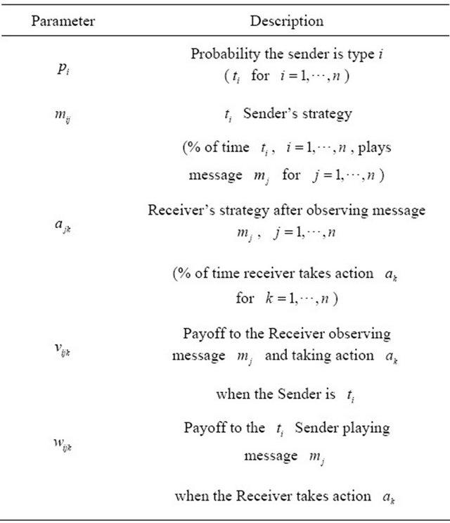
possible actions,  , that it chooses from its discrete strategy set once it observes the Sender’s message. Descriptions and definitions of the parameters in the
 ![]() -type signaling game are shown below.
-type signaling game are shown below.
Let us summarize the strategies played by the Sender and the Receiver, respectively, in vector form as
and
Note that ![]() is indexed differently than
is indexed differently than![]() . The first part of the index on
. The first part of the index on  refers to the Sender type and the second part refers to the message transmitted by the Sender. The first number in the index on
  refers to the message of the Sender, whereas the second stands for the action of the Receiver. This ordering is consistent with the order in which the nodes appear in the decision trees presented throughout the remainder of the paper.
The strategy  for the Sender can be interpreted as the conditional probability
  that the
  Sender will transmit message
 . Analogously, the strategy
  for the Receiver can be interpreted as the conditional probability
 .
.
We use a decision tree approach to identify Nash equilibrium strategies in signaling games. We first consider the case where neither player has any dominated strategies at Nash equilibrium and address the equilibrium calculation task. In this situation, the payoffs are structured so that there is an equilibrium where each type of Sender plays a mixture of all of its possible messages, so each Sender strategy satisfies  at Nash equilibrium. Correspondingly, the payoffs are also structured so that the Receiver plays a mixture of all its possible strategies after observing each message, which requires each Receiver strategy to satisfy
 .
.
By inspecting the decision tree models, we are able to intuitively observe the conditions that must exist for a solution to be a Nash equilibrium. The decision tree provides for easy calculation of the expected values for each player, which are ultimately used to derive the mathematical conditions necessary for a Nash equilibrium in purely mixed strategies.
3. Signaling Game Example
This section analyzes a two-type signaling game. For now, we assume nature’s selection of each Sender type is equally likely, i.e. . The Sender will choose one of two messages-Left or Right. The selection of the Left strategy by the
  Sender is the strategy
 , whereas the choice of Left for the
 ![]() Sender is
Sender is . The alternate strategies (Right) are denoted by
  and
and  for
for  and
and![]() , respectively, and these probabilities satisfy
, respectively, and these probabilities satisfy  and
and .
.
Once the Receiver observes the signal, it decides whether or not to move Up or Down and this threat represents its strategy. If it observes the Left message, its Up strategy is denoted by . If it observes Right, its Up strategy is denoted by
 . A Down strategy by the Receiver is denoted by either
  or
or , depending on the type of signal observed.
The payoffs for the Sender and Receiver are shown in Table 1. As an example, if the Receiver moves Up against a  Sender, both players could suffer significant losses, thus
  and
and . The Sender ends up with a worse outcome in this scenario by selecting Right, so
 .
.
3.1. Receiver’s Nash Equilibrium Strategies
The decision tree for the Sender in this game is shown in the left panel of Figure 1. The model shows that nature chooses the Sender’s type. After learning its type, the Sender chooses its message. Whereas the “Type” node is a chance node, the “Signal” nodes are random strategy nodes as defined by Cobb and Basuchoudhary [14], as the probabilities at these nodes represent Sender strategies. These nodes are shaded to distinguish them from typical chance nodes. After its strategy is chosen, the Sender’s payoff in the game is determined by the action chosen by the Receiver.
To find its Nash equilibrium strategies, the Receiver rolls back the Sender’s decision tree one level as shown in the left panel of Figure 2. Since all nodes in the tree are chance nodes, the roll-back procedure involves calculating expected values. For example, the  Sender observing
  calculates its expected value as
  at the chance node representing the Receiver action at the top of its tree in Figure 1. This expected value is placed in the rolled back decision tree in Figure 2 as the payoff on the branch representing the
  Sender and the
  observation. Other expected values are calculated similarly during the roll-back process.
Two conditions must be met by the strategies ,
,  ,
,  , and
, and  established at Nash equilibrium by the Receiver:
1) A  Sender must be indifferent among all possible strategy assignments
  and
and .
.
2) A t2 Sender must be indifferent among all possible strategy assignments  and
and .
.
These conditions are met when the expected values at the end of either branch at the two Signal nodes in the decision tree in the left panel of Figure 2 are equal, or
Table 1. The payoffs to each player in the signaling game.
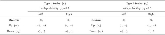
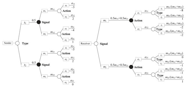
Figure 1. Decision trees for the general two-type signaling game.
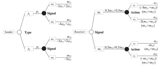
Figure 2. Decision trees rolled back one level.
when
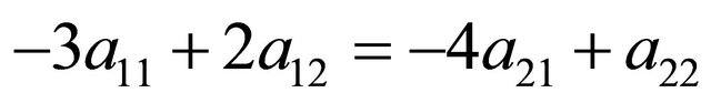
and
The solutions must also meet the conditions  and
and . The solution to this system of four equations in four unknowns is
 ,
,  ,
,  , and
, and .
.
The equilibrium calculation task is easily accomplished by solving the decision tree, because the expressions required to solve for ,
,  ,
,  , and
, and  are precisely the expected values calculated during rollback.
The strategies ,
,  ,
,  , and
, and  determined using this method are only guaranteed to make the Sender indifferent between any assignment of its strategies if none of its pure strategies is dominant. However, if a dominant strategy exists in the game, the decision tree solution can assist in the strategy selection task described in the introduction. For example, suppose the Sender’s payoffs in the example are changed so that
 . The solution process outlined previously yields
 . Since this not a valid probability, a purely mixed strategy equilibrium does not exist and the Sender must have at least one pure strategy at equilibrium.
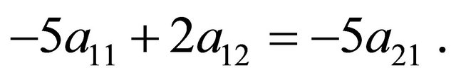
Observe from the tree in the left panel of Figure 1 (with  replaced by
 ) that
 ![]() should never move Left, so
should never move Left, so . Note from the Receiver’s tree in Figure 2 that with
 , when the Receiver observes
  it will never move Up
  because
 . The Receiver’s Nash equilibrium conditions are further reduced to
  and
and . The solution (
 and
and ) is given by Proposition 1 in Cobb and Basuchoudhary [14, p. 252].
3.2. Sender’s Nash Equilibrium Strategies
The decision tree for the Receiver in this game is shown in the right panel of Figure 1. The Receiver does not directly learn the Sender’s type, but does observe whether it chooses Left or Right. Once it observes this message, it decides whether to move Up or Down. The “Action” nodes are shaded to indicate these are random strategy nodes (as opposed to typical chance nodes). The payoff to the Receiver in the game is then determined by the Sender’s actual type.
The marginal probabilities for the Sender’s message type are calculated as
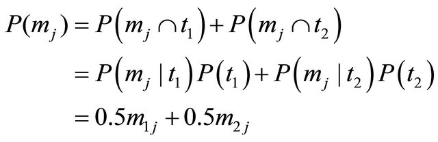
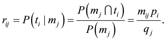
for . The conditional probabilities for the Sender’s type given the observed message in this model are determined using Bayes’ rule as
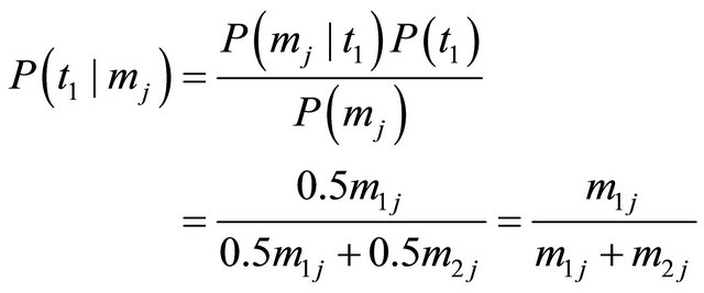
with .
.
To find its Nash equilibrium strategies, the Sender rolls back the Receiver’s decision tree one level as shown in the right panel of Figure 2. For example, the Receiver observing  and taking action
  calculates its expected value as
at the chance node representing the Sender type at the top of its tree in Figure 1. This expected value is placed in the rolled back decision tree in Figure 2 as the payoff on the branch representing the Receiver observing  and taking action
 .
.
Two conditions must be met by the strategies ,
,  ,
,  , and
, and  established at Nash equilibrium by the Sender:
1) If the Receiver observes , it must be indifferent between the strategies
  and
and .
.
2) If the Receiver observes , it must be indifferent between the strategies
  and
and .
.
These conditions are met when the expected values at the end of either branch at the two Action nodes in the decision tree in the right panel of Figure 2 are equal, or when
and
The solutions must also meet the conditions 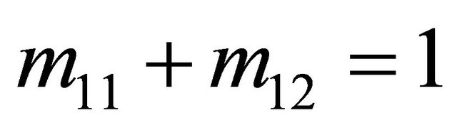 and
and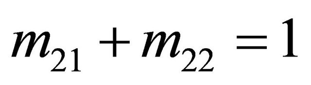 . Solving this system of four equations in four unknowns gives
 ,
,
 ,
,  , and
, and .
.
The strategies ,
,  ,
,  , and
, and  determined using the process outlined above are only guaranteed to make the Receiver indifferent between any assignment of its strategies if none of its strategies are dominant. Recall the example from the last section where the Sender’s payoffs are such that it always plays
  and
and . The revised probabilities in the Receiver’s decision tree will indicate that
 . We also established that in this scenario the Receiver observing
  should always play
  and
and . By inserting the pure strategies that will always be played by both the Sender and Receiver in the decision trees and rolling back the trees, the Nash equilibrium strategies for a semi-separating equilibrium can be determined. The solution for the Receiver observing
  is given by Proposition 2 in Cobb and Basuchoudhary [14, p. 252].
In this next section, decision trees and the expected values obtained from the solution process are used to obtain a pure mixed strategy Nash equilibrium for the ![]() -type signaling game.
-type signaling game.
4. General Signaling Game
In this section, we discuss the general ![]() -type signaling game. Decision trees similar to those used in the
-type signaling game. Decision trees similar to those used in the  case will be useful in demonstrating the conditions that are required to establish a Nash equilibrium.
4.1. Analysis of Sender’s Decision Tree
Figure 3 shows a portion of the decision tree for the Sender in this game. The model is expanded beyond the
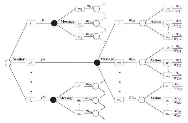
Figure 3. Sender’s decision tree in the general signaling game.
“Message” branch for the ![]() Sender. This expansion shows that the
Sender. This expansion shows that the ![]() Sender chooses from among
Sender chooses from among ![]() possible messages. Once it selects a message, it will which of the Receiver’s
possible messages. Once it selects a message, it will which of the Receiver’s ![]() possible actions has been taken. An expansion of the decision tree for the other Sender types would appear similarly.
possible actions has been taken. An expansion of the decision tree for the other Sender types would appear similarly.
Rolling back the section of the decision tree in Figure 3 for the ![]() Sender results in the expected values
Sender results in the expected values
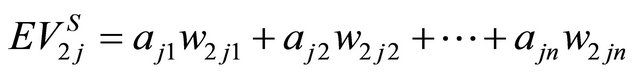
for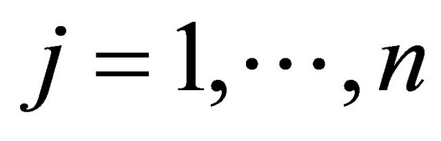 . A Nash equilibrium in this game must meet the
  separate conditions
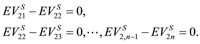 (1)
(1)
More generally, the Receiver’s strategies at Nash equilibrium must obey the conditions
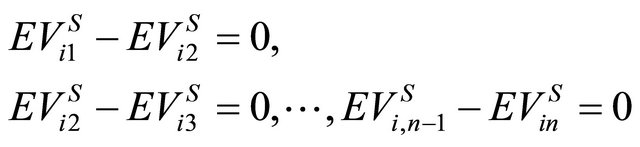 (2)
(2)
for .
.
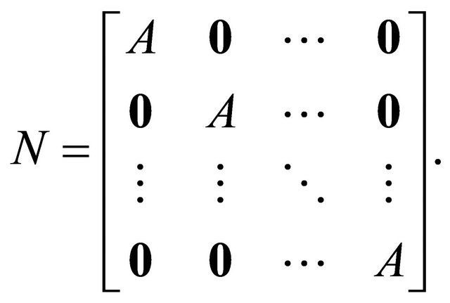
To solve for the mixed strategy Nash equilibrium strategies for the Receiver, we construct the  matrix
  as
as
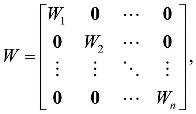
where each  is itself an
 ![]() matrix and 0 is the
matrix and 0 is the ![]() zero matrix. The
zero matrix. The , kth entry of block
  is simply
 . The vector
  is
is , with

Note that .
.
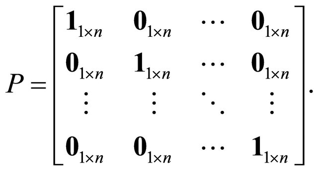
We can encode the conditions specified in (1) and (2) in the  matrix
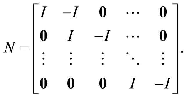
where  is the
 ![]() identity matrix.
identity matrix.
To satisfy a Nash equilibrium, we need  =
=  This gives us
  equations for our
  unknowns. We have yet to use the fact that the sum of the
  should be one (when j is fixed). The
matrix  takes this into account:
Thus, we want . Let
. Let 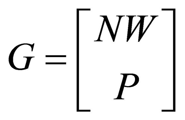 and define
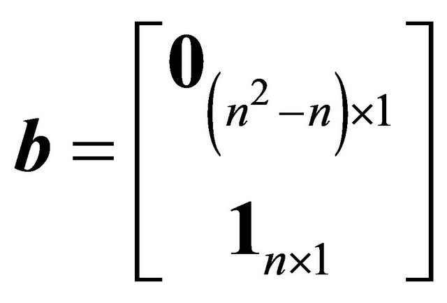 . We want to solve for
 ![]() in the equation
in the equation
Thus, the Nash equilibrium strategies for the Receiver are determined as
provided these entries are all non-negative. When the Receiver plays the strategies in , the Sender cannot unilaterally change its strategy to earn a higher expected payoff.
The prior discussion describes how the decision tree formulation is used for equilibrium calculation in the case of a purely mixed strategy equilibrium. To aid in strategy selection, the vector ![]() can be examined to determine whether there are any dominated strategies at equilibrium. This is indicated when
can be examined to determine whether there are any dominated strategies at equilibrium. This is indicated when ![]() contains entries that are not strictly between 0 and 1, or when
contains entries that are not strictly between 0 and 1, or when  is not invertible. In the
 ![]() -type signaling game, if a Sender of any type has any dominated strategies, these should be assigned zero probabilities prior to finding the remaining strategies in
-type signaling game, if a Sender of any type has any dominated strategies, these should be assigned zero probabilities prior to finding the remaining strategies in ![]() that comprise the Receiver’s strategies in a Nash equilibrium. Since the Receiver can assume that the Sender will never play dominated strategies, it can adjust its strategies accordingly and may find dominated strategies of its own. The decision tree methodology can still be useful in determining Nash equilibrium strategies for the Receiver. A well-defined algorithm for finding Nash equilibria where each player chooses some pure strategies and mixes over the remaining strategies is beyond the scope of this paper and requires future research. An example of such a solution in the context of a specific example will be provided later in this section.
that comprise the Receiver’s strategies in a Nash equilibrium. Since the Receiver can assume that the Sender will never play dominated strategies, it can adjust its strategies accordingly and may find dominated strategies of its own. The decision tree methodology can still be useful in determining Nash equilibrium strategies for the Receiver. A well-defined algorithm for finding Nash equilibria where each player chooses some pure strategies and mixes over the remaining strategies is beyond the scope of this paper and requires future research. An example of such a solution in the context of a specific example will be provided later in this section.
4.2. Analysis of Receiver’s Decision Tree
The Receiver’s decision tree in the general ![]() -type signaling game is partially shown in Figure 4. This diagram shows the detail in the tree beyond the “Action” node when the Receiver observes message
-type signaling game is partially shown in Figure 4. This diagram shows the detail in the tree beyond the “Action” node when the Receiver observes message . The detail shows that the Receiver will first learn the message selected from the Sender’s
 ![]() possible choices. Once it
possible choices. Once it
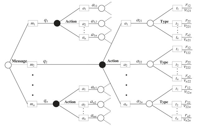
Figure 4. Receiver’s decision tree in the general signaling game.
observes the message, it chooses an action from its ![]() available possibilities. Only after the Receiver selects an action does it finally learn which of the
available possibilities. Only after the Receiver selects an action does it finally learn which of the ![]() possible Sender types it opposes in the game.
possible Sender types it opposes in the game.
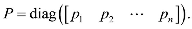
In this section,  is an
is an ![]() diagonal matrix that holds the probabilities
diagonal matrix that holds the probabilities  on the diagonal, or
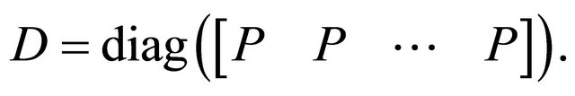
 Let
Let  be the
diagonal matrix of ![]() copies of
copies of , or
, or
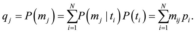
The marginal probabilities for the message observed by the Receiver are calculated as
The conditional probabilities for Sender type given the message observed by the Receiver are calculated as
where ![]() is the conditional probability the Sender is
is the conditional probability the Sender is  given message
  is observed. Let
Note that  is indexed in the same manner as
![]() .
.
One can derive  from
from ![]() by pre-multiplying
by pre-multiplying ![]() by the above matrix
by the above matrix  and by the matrix
  defined as the
  diagonal matrix whose first
 ![]() diagonal entries are
diagonal entries are , whose second
 ![]() diagonal entries are
diagonal entries are![]() , etc. One can view
, etc. One can view  as being block diagonal,
 where each
  is
is ![]()
diagonal, with the diagonal containing only![]() . We have that
. We have that . However, in calculating the Nash equilibrium strategies, we will not actually need the
 ’s and hence we will not need
 . The matrix
  will be used to calculate the expected value in the game for the Receiver.
 is
is  and contains the Receiver’s payoffs. It is analogous to the matrix
  from previous analysis of the Sender’s tree, but is defined in a different manner. It can be viewed as a diagonal block matrix,
where each  is
is![]() , and the
, and the  entry of
  is
is .
.
Let  denote the
  vector of expected values of the outcomes for the Receiver, or

Note the indexing of  differs from
 . The components of
  are derived by rolling back the decision tree in Figure 4. For instance, rolling back the tree for the Receiver observing
  results in the following expected values:
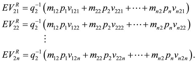
In general, we have . At Nash equilibrium, the Receiver observing the message
  must be indifferent between each of its actions, so that
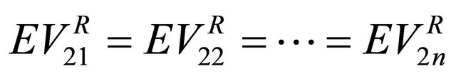 .
.
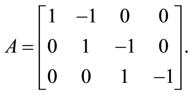
The matrix  will be
  with
with
with  an
an  “upper bidiagonal” matrix, with 1s on the diagonal and −1s on the upper bidiagonal. For instance, in the
  case, we have
We have .
.
Replacing  with
with  gives
gives . Because of the block diagonal structure of
  and
and , we have that
 . Likewise,
  , where
 is
is  diagonal, with
  copies of each
 ![]() on the diagonal instead of
on the diagonal instead of ![]() copies.
copies.
Thus
Since  is invertible (as long as no
 ), this implies that
 , and hence we can ignore
  and directly solve for
![]() .
.
We currently have  equations describing our
  unknowns. Our final
 ![]() equations come from the fact that the
equations come from the fact that the  form a distribution, hence
for . Because of the way that we have indexed the matrix
![]() , this amounts to summing every
, this amounts to summing every  entry of
 ![]() and getting 1. This can again be done conveniently through matrix multiplication.
and getting 1. This can again be done conveniently through matrix multiplication.
Let S be the  matrix which is the concatenation of
 ![]() copies of the
copies of the ![]() identity matrix
identity matrix . That is,
 . Then
 .
.
Let . We want to solve for
 ![]() in the equation
in the equation
where  is defined as in the previous section. Thus, the Nash equilibrium strategies for the Sender are determined as
We can show an example of the conditions under which  will not be invertible. If for two values of
 , say
, say  and
and , we have that
  and
and , then
  will have two identical columns and hence will not be invertible.
In the ![]() -type signaling game, if a Receiver observing any message has any dominated strategies, these should be assigned as zero in any Nash equilibrium solution. This may occur simply because of the structure of the Receiver’s payoffs, or perhaps because the Receiver can assume that at least one type of Sender has dominated strategies that will never be played at Nash equilibrium. One such case mentioned earlier occurs when the Receiver has multiple actions that lead to exactly the same payoffs (this causes
-type signaling game, if a Receiver observing any message has any dominated strategies, these should be assigned as zero in any Nash equilibrium solution. This may occur simply because of the structure of the Receiver’s payoffs, or perhaps because the Receiver can assume that at least one type of Sender has dominated strategies that will never be played at Nash equilibrium. One such case mentioned earlier occurs when the Receiver has multiple actions that lead to exactly the same payoffs (this causes  to be invertible). All but one of such strategies can be considered dominated and assigned zero probabilities. As stated in the previous section, some additional discussion will be provided later in the paper regarding the use of decision trees to identify such equilibria, and further study of methods for using decision trees to solve for such equilibria will be the subject of ongoing research.
The same conclusions to those in Section 3 for the two-type signaling game about the solutions  and
and  outlined above can be made for the
 ![]() -type signaling game. The solutions either compute a purely mixed Nash equilibrium or indicate that a Nash equilibrium containing at least some pure strategies exists.
-type signaling game. The solutions either compute a purely mixed Nash equilibrium or indicate that a Nash equilibrium containing at least some pure strategies exists.
5. Examples
In this section, the process from Section 4 is used to find Nash equilibrium strategies in the signaling game from Section 3 with .
.
5.1. Determining the Receiver’s Nash Equilibrium Strategies
In this problem, let . Substituting the values from Table 1 gives
Recall that  At Nash equilibrium
 and
and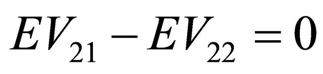 . This idea is encoded in the matrix
 . Combining
  and
and  gives
gives
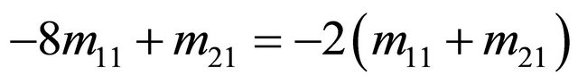
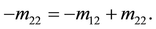
 (3)
(3)
Therefore,
 (4)
(4)
Up to this point, we have two equations for four unknowns. The sum of the  should be one (when
  is fixed). This is ensured by the matrix
 . Thus, we have that
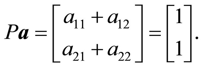 (5)
(5)
Combine Equations (4) and (5) together. The matrices  and
and  are both
 , and hence the matrix
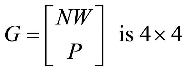
and
The Nash equilibrium strategies are
5.2. Determining the Sender’s Nash Equilibrium Strategies
This section illustrates the determination of the Sender’s solution in the example from Section 3.
Let the Sender’s strategy vector be denoted by
 and the vector of revised probabilities
  be denoted by
 The matrix
  holds the probabilities
  on the diagonal. The matrix
  is
is  block diagonal, with two copies of
  on the diagonal.
The matrix  contains the payoffs
  and is also block diagonal,
  , or
, or
The  entry of
  is
is . Thus,
 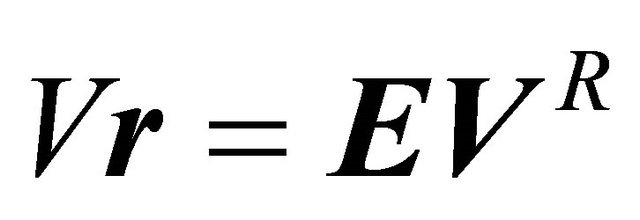 where
where 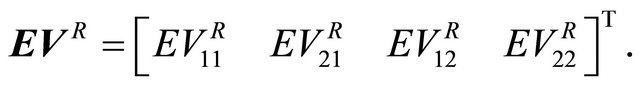 We want to multiply
  by a matrix
  that ensures we have a Nash equilibrium. This matrix is the same as
  from the previous section.
The expression  gives two equations for our four unknowns. Two more equations are required because
 ![]() represents two probability distributions where
represents two probability distributions where . Let
. Let . The matrix
 ![]()
is formed such that . This gives two more equations that must be satisfied at Nash equilibrium.
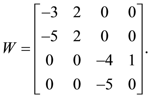
We form  as before, concatenating our matrices.
Set . Thus
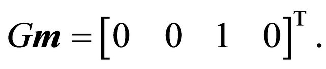
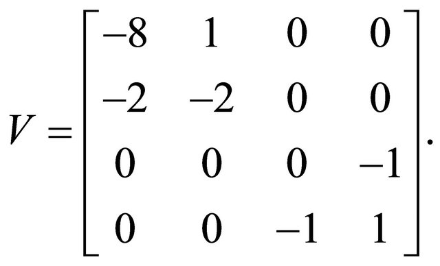
Forming  as directed gives
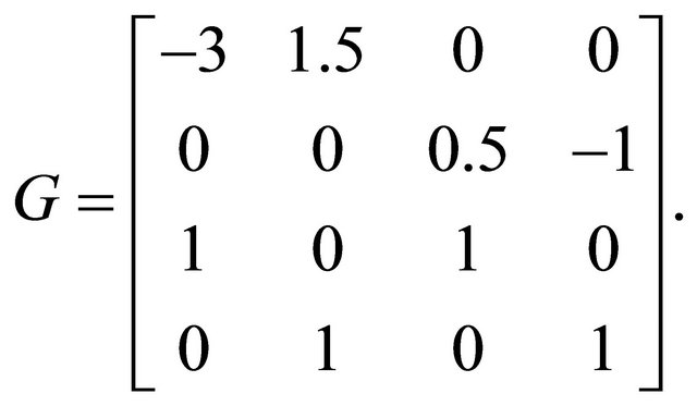
Finally, with  invertible,
 ![]() can easily be found. With this, the
can easily be found. With this, the ’s can be easily determined as can
  if needed.
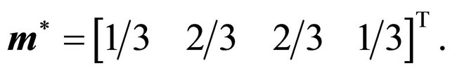
The Nash equilibrium strategies are
5.3. Nash Equilibria without Purely Mixed Strategies
When applied to an arbitrary set of Sender and Receiver payoffs, the solutions  and
and  can be classified into two mutually exclusive categories:
1) All elements of  and
and  are valid, non-zero probabilities (requiring that the matrices
  used to determine the solution are both invertible), i.e. the solution is a purely mixed Nash equilibrium.
2) Some or all elements of  and
and  are not valid non-zero probabilities, or one or both of the vectors of solutions are not defined because one of the
  matrices is not invertible.
All signaling games have either a pooling, separating, semi-separating or purely mixed Nash equilibrium. These equilibrium types are mutually exclusive. Solutions  and
and  from the first category above are identically associated with games with purely mixed strategies. Therefore, solutions from the second category above are identified with pooling, separating, or semi-separating equilibria. Thus, we can be certain that our solution technique will either identify a purely mixed strategy or verify the existence of a Nash equilibrium containing at least some pure strategies (the strategy selection task). In terms of the equilibrium calculation task, purely mixed strategy equilibria are the primary focus of this paper. We give an example in this section that uses decision trees to facilitate the determination of an equilibrium in the second category.
The payoffs and prior probabilities for Sender type in the game are listed in Table 2. The Sender may be one of three types and the Receiver has three possible actions. The first number in each pair is the payoff to the Receiver and the second number is the payoff to the Sender.
In this problem, calculating  or
or  in the strategy selection phase reveals that a purely mixed Nash equilibrium does not exist and dominated strategies must be identified to determine the Nash equilibrium. The procedure from Section 4 gives the solutions
 ,
,  , and
, and  as the strategies for the Receiver observing
 . Clearly, these are not probabilities and this result provides an indication that the Sender has a dominated strategy.
The part of the Sender’s decision tree related to the  Sender is shown in the left part of Figure 5 and rolled back in the right part of Figure 5. Again, the roll-back procedure involves calculating expected values. For instance, the
  Sender selecting
  obtains expected value
 . From these diagrams, we can clearly observe that the Sender will always play
 , as this strategy is dominated by both
  and
and . Specifically,

and
Once the Receiver accounts for the fact that , it will adjust its payoffs and ascertain (through similar analysis as that performed above for the Sender) that it should always play
  because
  is dominated by
  and
and .
.
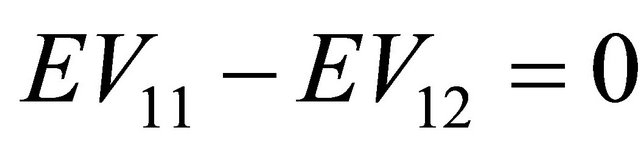
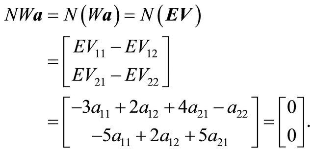
The method presented in Section 4 can be adapted to find the remaining equilibrium strategies in this game. Since , the expected value
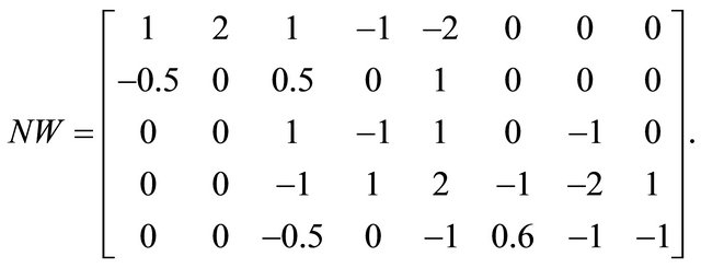
  does not have to be considered in the Nash equilibrium conditions when the Receiver determines its optimal strategies using the Sender’s decision tree. Since the first row of the matrix NW in (3) captures the condition
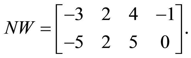
 , this row can be removed from the matrix. Since
  the second column of NW can be removed. The matrix is
The Nash equilibrium strategies for the Receiver (with  replaced) are

To determine its equilibrium strategies, the Sender must adjust the Receiver’s decision tree for the conditions
 and
and . After adapting the process in Section 4 for these dominated strategies, solving
 gives
gives

The strategy  has been re-added to the vector.
The decision tree for the Receiver observing  is shown in Figure 6 with the optimal strategies and resulting conditional probabilities for both players inserted. The Sender’s strategies make the Receiver indifferent between any possible assignment
  and
and  (although it has selected
  and
and  at equilibrium). Since
 , the Receiver can never gain a higher payoff by assigning any positive probability
 , so this was set to
  prior to determining the other equilibrium strategies.
This example demonstrates that the decision trees are still useful for identifying Nash equilibria that are not purely mixed (the strategy selection task). The process for interpreting the results of Section 4 for an arbitrary signaling game where a purely mixed Nash equilibrium does not exist, then adapting the matrices representing the Nash equilibrium conditions is not well-defined and has only been demonstrated by example. Creating such an algorithm requires further investigation, but the decision tree approach appears to hold promise for developing a heuristic approach to determining a Nash equilibrium in signaling games.
6. Conclusions
The main contribution of this paper is to introduce a standard approach to constructing and solving the equa-
Table 2. Payoffs to each player in the example.
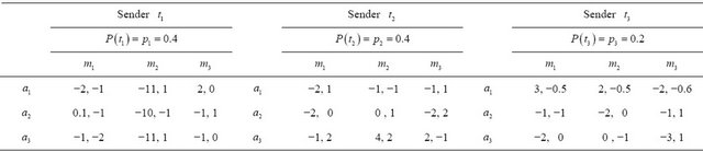
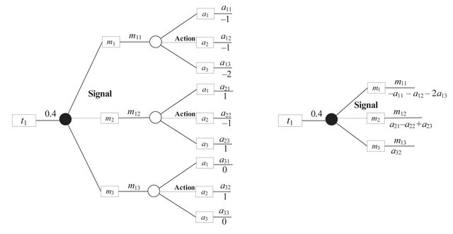
Figure 5. Decision tree for the t1 Sender.

Figure 6. Decision tree for the Receiver observing m1.
tions required to determine a mixed strategy Nash equilibrium in a signaling game. Some existing algorithms in the literature can solve two-type signaling games very fast. The problem is that once the game becomes even slightly more complex, finding equilibrium becomes increasingly difficult. This is acknowledged, for instance, by the developers of the Gambit software package [7].
In some sense, the purely mixed strategy is the most general solution for the n-type signaling game. Naturally, many signaling games have payoffs structured so that certain strategies for either player are dominated. In these cases, the decision tree can still be used to identify the Nash equilibrium conditions and solve for a mixed equilibrium over the remaining strategies. The eventual goal of future research is to provide new heuristic approaches for solving signaling games that can be derived from the solutions to the equations for the mixed strategy Nash equilibrium. This potential was demonstrated in Section 5.3 through an example where the Sender has a dominated strategy.
Decision trees provide a convenient modeling tool to facilitate the calculation of purely mixed Nash equilibria in signaling games. This paper extends decision tree results for the two-type signaling game presented by Cobb and Basuchoudhary [14] by finding general results for a purely mixed Nash equilibrium. Most game theory textbooks limit the possible types of solutions to pooling, separating, and semi-separating equilibria. The decision tree allows an analyst to simply compute a purely mixed Nash equilibrium, as opposed to testing a hypothesized Nash equilibrium by abstractly examining the payoffs or game tree for the problem.
The graphical representation of the decision tree models used to determine the purely mixed strategy Nash equilibria will clearly grow exponentially as the number of Sender types expands in the symmetric signaling game. However, the expected values required to solve such a decision tree are easily defined in matrix form. In a sense, we can dynamically construct nodes of interest in the decision tree, calculate expected values, then find the Nash equilibria using these expected values. This allows the decision tree solution to be used to find the purely mixed Nash equilibrium solution, even when the Sender has many possible types.
REFERENCES
- A. M. Spence, “Job Market Signaling,” Quarterly Journal of Economics, Vol. 87, No. 3, 1974, pp. 355-374. doi:10.2307/1882010
- P. Milgrom and J. Roberts, “Limit Pricing and Entry Under Incomplete Information: An Equilibrium Analysis,” Econometrica, Vol. 50, No. 2, 1982, pp. 443-459. doi:10.2307/1912637
- D. M. Kreps and J. Sobel, “Signalling,” In: R. J. Aumann and S. Hart, Eds., Handbook of Game Theory: With Economics Applications, Elsevier, Amsterdam, Vol. 2, No. 11, 1994, pp. 849-868.
- J. G. Riley, “Silver Signals: Twenty-Five Years of Screening and Signaling,” Journal of Economic Literature, Vol. 39, No. 2, 2001, pp. 432-478. doi:10.1257/jel.39.2.432
- B. von Stengel, “Equilibrium computation for TwoPlayer Games in Strategic and Extensive Form,” In: N. Nisan, T. Roughgarden, E. Tardos and V. V. Vazirani, (Eds.), Algorithmic Game Theory, Cambridge University Press, New York, 2007, pp. 53-78. doi:10.1017/CBO9780511800481.005
- N. Nisan, T. Roughgarden, E. Tardos and V. V. Vazirani, “Algorithmic Game Theory,” Cambridge University Press, New York, 2007. doi:10.1017/CBO9780511800481
- R. D. McKelvey, A. M. McLennan and T. Turocy, “Gambit: Software Tools for Game Theory, Version 0.2010.09.01,” 2011. http://www.gambit-project.org
- D. Rios Insua, J. Rios and D. Banks, “Adversarial Risk Analysis,” Journal of the American Statistical Association, Vol. 104, No. 486, 2009, pp. 841-854. doi:10.1198/jasa.2009.0155
- G. S. Parnell, C. M. Smith and F. I. Moxley, “Intelligent Adversary Risk Analysis: A Bioterrorism Risk Management Model,” Risk Analysis, Vol. 30, No. 1, 2010, pp. 32-48. doi:10.1111/j.1539-6924.2009.01319.x
- E. Paté-Cornell and S. Guikema, “Probabilistic Modeling of Terrorist Threats: A Systems Analysis Approach to Setting Priorities among Countermeasures,” Military Operations Research, Vol. 7, No. 4, 2002, pp. 5-20. doi:10.5711/morj.7.4.5
- D. Fudenberg and J. Tirole, “Game Theory,” MIT Press, Cambridge, 1993.
- D. M. Kreps and R. Wilson, “Sequential Equilibria,” Econometrica, Vol. 50, No. 4, 1982, pp. 863-894. doi:10.2307/1912767
- J. H. van Binsbergen and L. M. Marx, “Exploring Relations between Decision Analysis and Game Theory,” Decision Analysis, Vol. 4, No. 1, 2007, pp. 32-40. doi:10.1287/deca.1070.0084
- B. R. Cobb and A. Basuchoudhary, “A Decision Analysis Approach to Solving the Signaling Game,” Decision Analysis, Vol. 6, No. 4, 2009, pp. 239-255. doi:10.1287/deca.1090.0148
NOTES
*Corresponding author.