ABSTRACT

When inputs in the firm’s production function are pair-wise complements, I show that all variable factors of the firm are output elastic. Via Silberberg’s analysis, this implies that for given output of a competitive firm that marginal cost will rise more than average cost for a factor price increase. Accounting for changes in output through profit maximization and industry equilibrium change in output price, I show that cost pass-through can be larger than one in a competitive industry when inputs are complementary. Because input complementarity seems likely with commodity aggregates like materials, labor, energy, and capital, this could provide an alternative explanation for over cost shifting in commodity-oriented industries like the oil industry and food industries. This approach also allows researchers to abandon the highly restrictive assumption of constant elasticity of demand function facing the firm that is required under imperfect competition with constant marginal costs.

1. Introduction

The concept of output elasticity (percentage change in input usage for one percent change in output, holding factor prices constant) plays a prominent role in the theory of the firm. Among other things, the concept is useful in determining whether a firm will increase or decrease its output in response to a change in factor price [1]. There is also an important link between the output elasticity and elasticity of marginal cost with respect to a change in input price (holding output constant). That is, theelasticity of marginal cost with respect to a change in input price equals the product of output elasticity and cost share of the factor in total revenue. To see this, consider the firm producing a single output, y, with a set of n-inputs with the production function, where the n-th input is assumed to be a fixed factor. The effect of a change in the i-th factor price on marginal cost of output is [2]

(1)

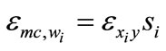
where is the firm’s cost function and subscripts denote partial derivatives. In the last step of Equation (1) use has been made of Shephard’s lemma. Converting Equation (1) to elasticitieswe obtain

(2)

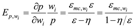
where 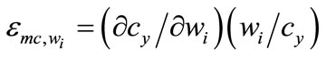is the elasticity of marginal cost with respect to a change in the i-th factor price, 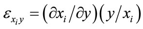is the output elasticity of the i-th factor, and 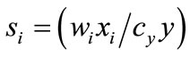is the share of total cost of the i-th factor in output valued at marginal cost. When the firm is a price taker, s_i is cost share of the i-th factor in total revenue; when the firm is imperfectly competitive in the output market, 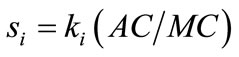, where 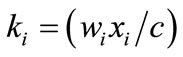is the total cost of the i-th factor as a share of total cost, 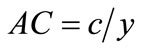is average cost, and MC is marginal cost.

Equation (2) shows there is a one-to-one relationship between the elasticity of marginal cost with respect to factor price and its output elasticity. The elasticity of marginal cost with respect to w_i will be larger (smaller) than s_i according as is larger (smaller) than 1. In general, we cannot say with certainty what the relationship will be. If the firm is in long-run equilibrium, where marginal cost equals average cost, then 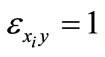and 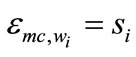[1]. If the production function is homothetic and there is decreasing returns to scale then 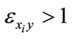for all variable factors so that 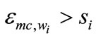[2]. In what follows, I establish that such a relationship can be expected to hold generally if we only impose the less restrictive condition of input complementarity. Input complementarity is a reasonable assumption when dealing with aggregate inputs like labor, materials, energy, and capital. This assumption also plays a crucial role in supermodularity and monotone comparative statics [3]¹.

2. The Basic Result

Linear homogeneity of the long-run production function is a reasonable assumption in light of the replication argument [5]. Linear homogeneity implies the production function has the form for. Without loss in generality, assume that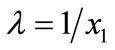. Then the production function can written as

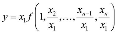. (3)

In this form, the production function can be used to determine the output elasticity of any variable factor.

In the short run with x_n fixed, assume the firm is a price taker in both output and factor markets. Assume also that the firm takes x₁ as fixed in determining its profit-maximizing input levels². The first-order conditions for profit maximization conditional on x₁ are:

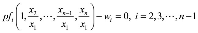. (4)

Solving these n – 2 equations for the conditional input demand functions yields:

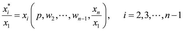. (5)

Substituting these functions into the production function yields the conditional supply function

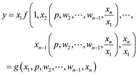. (6)

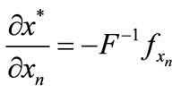
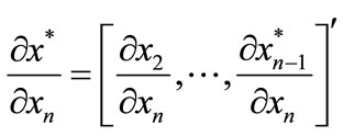
Differentiating Equation (6) with respect to x₁ yields the expression

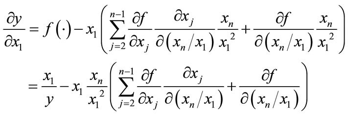
This expression implies that

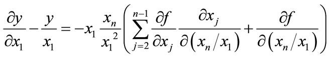. (7)

This has implications for the output elasticity of x₁, which can be determined through substituting the optimal output-constant demand function for x₁, 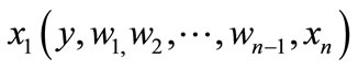, into Equation (6) to obtain the identity

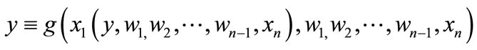
where now y is assumed to be the profit-maximized value for output. Differentiating the identity with respect to y:

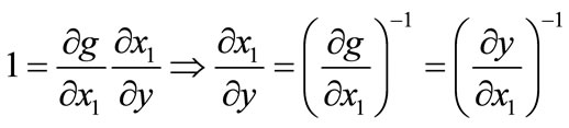
Thus,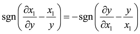. This means that if the sign of Equation (7) is negative, then and the output elasticity.

Theorem

When inputs are complementary in production, all output elasticities of the firm will be larger than one.

Proof. Let

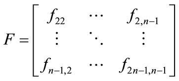
be the Hessian of the production function with respect to from differentiating the firstorder conditions in Equation (4). The comparative statics of the n – 2 conditional input demand functions can be characterized as follows:

(8)

where

and .

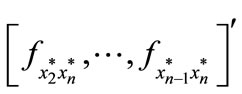
The solutions in Equation (8) can be written more explicitly as follows:

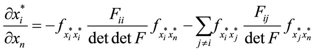(9)

where is the co-factor of in F. The term 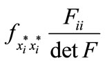is negative because F is a negative definite matrix for the firm to maximize profit. Because the matrix F is a Metzler matrix (off-diagonal elements nonnegative and diagonal elements nonpositive), each of the terms will be nonpositive [6]. This means when 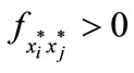for all i and j, (i.e., input complementarity) that each term of the solution to Equation (8) as shown by Equation (9) will be positive. Thus,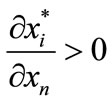. Noting that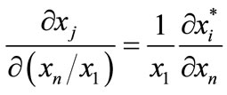, we have immediately from Equation (7) that 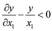so that 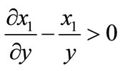and the output elasticity.

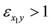3. Implications for Cost Pass-Through

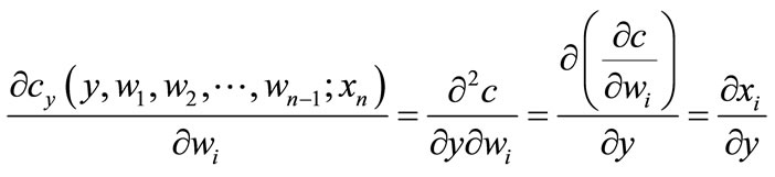
From Equation (2) we also see that an output elastic factor demand implies that the elasticity of marginal cost from an increase in factor price will be greater than the cost of the input as a share of total revenue. This result, while important in its own right, is only valid if output remains constant. To calculate the price effect we must account for the effect the change in factor price has on output as well.

In the identical firm case, the comparative static expression for cost pass-through for a competitive market in the short run can be shown to equal³

(10)

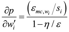
where is the elasticity of output price with respect to the i-th factor price, ε is the supply elasticity, and is the demand elasticity of the output. It is useful for our purpose to normalize Equation (10) by redefining the elasticity of price transmission as

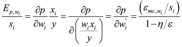. (11)

This expression now shows how much output price changes for each unit output change in the i-th factor price. For example, if the input is crude oil and output is gasoline, the expression in Equation (11) now shows how much the price of gasoline changes for a change in the price of crude oil per gallon of gasoline.

Equation (11) indicates that cost pass-through can now be larger than 1. This will occur when 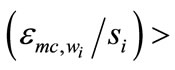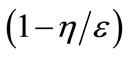. This will more likely be the case the larger the supply elasticity relative to the absolute value of the demand elasticity.

To see how plausible cost pass-through larger than 1 can be, consider the cost function derived from the CobbDouglas short-run production function:

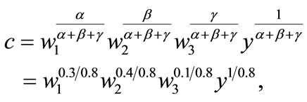
where the parameters and represent the cost shares of the three variable inputs with returns to scale equal to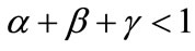. The values chosen are typical of many manufacturing industries for materials, labor, and energy⁴. The output elasticity for the material input in this case (which equals that for labor and energy because production function is homothetic in this case) is 1/0.8 = 1.25. The value for 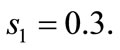The elasticity of marginal cost with respect to output is 1/0.8 – 1 = 0.25. Thus, the supply elasticity is ε = 1/0.25 = 4. If the demand elasticity is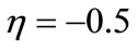, then the output price change from a one unit change in materials price per unit output is

.

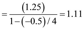
So even with a very elastic supply curve, about 11% more of the increase in materials price would be passed on to output price.

4. Conclusions

In the general case of input complementarity in production, I have shown that output elasticities of all variable factors will be elastic. A direct implication of this finding is that with input complementarity, marginal cost will increase more than average cost for an increase in factor price. For somewhat aggregate inputs like labor, materials, energy, capital, we would expect input complementarity to be the rule rather than the exception. It is also noteworthy that the result does not depend on any other restrictions on the production function other than the long-run production function exhibiting constant returns to scale. Another condition leading to this result is homotheticity of the short-run production function [2]. Homotheticity is a special case of the theorem derived here and would require that not only each factor be output elastic but that all of the output elasticitiesbe equal. The only constraint on the relative magnitudes of the output elasticities when inputs are complements in production is that the share-weighted sum of the output elasticities equals the ratio of marginal cost to average cost [8]

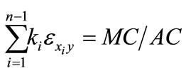where recall that k_i is the total cost of the i-th factor as a share of total costs.

The main implication for cost pass-through is that we have an explanation based on the cost structure for how there can be more than full pass-through of costs. The usual explanation assumes marginal costs are constant so that cost pass-through depends on the shape of the demand curve. However, it is well-known that only very restrictive forms of the demand function will give rise to more than complete cost pass-through [9].

5. Acknowledgements

Research supported in part by the North Carolina Agricultural Research Service, Raleigh, North Carolina, 27695.

REFERENCES

NOTES

¹A function is said to be supermodular if it is increasing in first differences in for all i ≠ j with each x_h fixed for h ≠ i and h ≠ j. When the function is twice, continuously differentiable supermodularity is equivalent to 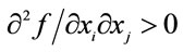for all i ≠ j with each x_h fixed with each x_h fixed for h ≠ i and h ≠ j [4]. Complementarity is therefore a direct implication of supermodularity.

²This should not be taken to imply that profit is not maximized with respect to x₁. Indeed, the level of x₁ considered could be its optimal value. The reason for optimizing profit conditional on x₁ is for analytical purposes to derive an explicit relationship between and when all the other variable factors are optimized.

³Let y = D (p) be the market demand function for the output and be the inverse market supply function (i.e., the condition that each firm produce where price equals marginal cost). Substituting the demand function for y in the inverse supply function, differentiating with respect to w₁, solving for, and converting to elasticities yields Equation (10). See [7] for a similar derivation in the context of evaluating cost pass-through for anti-trust cases.

⁴The numbers chosen here represent costs of producing and marketing food in the U.S. and are derived from values reported in USDA, ERS website http://www.ers.usda.gov/Data/FarmTo Consumer/Data/componentstable.htm. The materials category is agricultural raw materials plus packaging materials. The energy category is transport plus fuel and electricity costs. Labor costs represent all labor costs of processing agricultural raw materials into final food products.

REFERENCES

- E. Silberberg, “Theory of the Firm in ‘Long-Run’ Equilibrium,” American Economic Review, Vol. 64, No. 4, 1974, pp. 734-741.
- E. Silberberg, “The Structure of Economics: A Mathematical Analysis,” McGraw-Hill, Inc., New York, 1990.
- R. Amir, “Supermodularity and Complementarity in Economics: An Elementary Survey,” Southern Economic Journal, Vol. 71, No. 3, 2005, pp. 636-660. doi:10.2307/20062066
- D. Topkis, “Comparative Statics of the Firm,” Journal of Economic Theory, Vol. 67, 1995, pp. 370-401. doi:10.1006/jeth.1995.1078
- H. Varian, “Microeconomic Analysis,” W.W. Norton & Co., New York, 1992.
- J. Quirk, “Qualitative Comparative Statics,” Journal of Mathematical Economics, Vol. 28, 1997, pp. 127-154. doi:10.1016/S0304-4068(97)00800-8
- G. Kosicki and K. Cahill, “Economics of Cost Pass through and Damages in Indirect Purchases Antitrust Cases,” Antitrust Bulletin, Vol. 51, No. 3, 2006, pp. 599- 630.
- G. Hanoch, “Production and Demand Models with Direct or Indirect Implicit Additivity,” Econometrica, Vol. 43, No. 3, 1975, pp. 395-420. doi:10.2307/1914273
- J. Bulow and P. Pfleiderer, “A Note on the Effect of Cost Changes on Prices,” Journal of Political Economy, Vol. 91, No. 1, 1983, pp. 182-185. doi:10.1086/261135
NOTES
1A function  is said to be supermodular if it is increasing in first differences in
for all i ≠ j with each xh fixed for h ≠ i and h ≠ j. When the function is twice, continuously differentiable supermodularity is equivalent to
for all i ≠ j with each xh fixed with each xh fixed for h ≠ i and h ≠ j [4]. Complementarity is therefore a direct implication of supermodularity.
2This should not be taken to imply that profit is not maximized with respect to x1. Indeed, the level of x1 considered could be its optimal value. The reason for optimizing profit conditional on x1 is for analytical purposes to derive an explicit relationship between  and
and  when all the other variable factors are optimized.
3Let y = D (p) be the market demand function for the output and  be the inverse market supply function (i.e., the condition that each firm produce where price equals marginal cost). Substituting the demand function for y in the inverse supply function, differentiating with respect to w1, solving for
, and converting to elasticities yields Equation (10). See [7] for a similar derivation in the context of evaluating cost pass-through for anti-trust cases.
4The numbers chosen here represent costs of producing and marketing food in the U.S. and are derived from values reported in USDA, ERS website http://www.ers.usda.gov/Data/FarmTo Consumer/Data/componentstable.htm. The materials category is agricultural raw materials plus packaging materials. The energy category is transport plus fuel and electricity costs. Labor costs represent all labor costs of processing agricultural raw materials into final food products.