Journal of Mathematical Finance
Vol.3 No.1A(2013), Article ID:29356,7 pages DOI:10.4236/jmf.2013.31A022
Sequential Variable Selection as Bayesian Pragmatism in Linear Factor Models
1Department of Economics, University of Western Ontario, Ontario, Canada
2Department of Finance, University of Sydney, Sydney, Australia
3Department of Accounting and Finance, University of Greenwich, London, UK
Email: jknight@uwo.ca, ses999gb@yahoo.co.uk, zq03@gre.ac.uk
Received January 10, 2013; revised February 9, 2013; accepted February 20, 2013
Keywords: Linear Factor Models; Bayesian Statistics; Sequential Regression
ABSTRACT
We examine a popular practitioner methodology used in the construction of linear factor models whereby particular factors are increased or decreased in relative importance within the model. This allows model builders to customise models and, as such, reflect those factors that the client and modeller may think important. We call this process Pragmatic Bayesianism (or prag-Bayes for short) and we provide analysis which shows when such a procedure is likely to be successful.
1. Introduction
The purpose of this paper is to investigate statistical procedures frequently used by practitioners to build factor models. In particular, we are interested in the variable selection methodologies that are used to give a particular returns model a particular style and nature. For example, in the context of global models, one may wish the model to depend more or less upon domestic factors such as country’s indices rather than, say, global factors such as currency or world equity and bond markets. Likewise at the domestic level, one may want one’s model to be built around styles (value, growth etc.) rather than industries or sectors—alternatively, the opposite may be preferred. The literature on this topic is very sparse. We present a brief survey of alternative approaches. The problem can be viewed as a practical alternative to well-known Bayesian procedures, such as Jorion’s (1986) [1] Bayes Stein adjustment and Black-Litterman’s BL model (1991, 1992) [2,3]. These models are both examples of Bayesian adjustment which effectively updates currently held opinions with data to form new opinions. Satchell and Scowcroft (2000) [4] also present details of Bayesian portfolio construction procedures based on Black-Litterman models. The essential idea in this process is to have a prior distribution over expected returns or over the regression Betas. In either case, one needs to specify hyperparameters which are, in practice, very troublesome. The procedure we advocate, and which is used by practitioners, is to convert beliefs about the magnitude of betas into procedures of sequential regression.
In Section 2 we shall describe how this is done in practice and how it could be analysed in theory. In Section 3 we shall present conditions under which these methodologies should work. Section 4 presents some empirical results. Conclusions and further discussion are presented in Section 5.
2. Theorem
There are a number of procedures that can be used to facilitate one factor being preferred to another. Here we shall assume that our return series is denoted by the n × 1 vector y, and the two factors over which we may have preferences are denoted by  and
and  respectively, both n × 1 vectors.
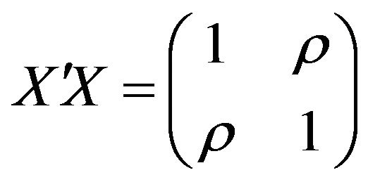
Letting![]() , we will facilitate calculations later by making the following assumption:
, we will facilitate calculations later by making the following assumption:
Our “true” model is
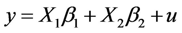 (1)
(1)
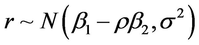
where y and u are n× 1 vectors, β1 and β2 are scalars and 
This is obviously a simplification of the general case, but little is lost in so doing and it allows us to focus on the essential features of the problem. We now define the sequential variable selection method (SVSM), which is the essential component of the prag-Bayes approach.
Definition: The SVSM is defined by the following procedure. If you want variable 1 to “explain” more of y asset returns than variable 2, you regress variable 1 first in a univariate regression. The coefficient for variable 2 is then calculated by regressing the residual of y on variable 1 upon the residual of variable 2 on variable 1.
The question we wish to ask is: under what circumstances will this procedure lead to a larger estimated exposure  of variable 1 versus that of variable 2,
 . A closely related question is the conditions under which the new slope estimates will be bigger or smaller than those calculated from conventional ordinary least squares (OLS).
It is worth discussing a variant on these procedures which concerns testing. Rather than just focusing on the magnitude of : we could also alternatively make inclusion and exclusion decisions based on t-statistics. Our results can be tilted in the desired direction by moving the critical values of our tests.
In terms of the Equation (1), we do not wish to impose β1 > β2 for all stocks. This is because we recognise that particular stocks may not be modeled subject to such a constraint. To illustrate, in the case of factor 1 being a global factor and factor 2 being a domestic factor, we can imagine cases of multinationals where β1 > β2 but there will also be Japanese railway stocks, for example, where the opposite is true. Accordingly, a Bayesian approach where β1 and β2 are variable allows us to approach this question in a theoretically appealing way.
We may have a prior, that P(β1 ≥ β2) ≥ d where d is some threshold probability, and P() denotes the probability of the event in brackets. This can be easily imposed by an adroit choice of hyper-parameters in the prior joint distribution of β1 and β2. Then we can compute the likelihood in the usual way, and finally, the posterior distribution of β1 and β2 where the posterior probability of β1 ≥ β2 can be computed in a straightforward manner. However, implementation of hierarchical Bayes models required a number of ancillary assumptions that are not particularly transparent, see Gelman (2004) [5] for example. We shall not detail how a Bayesian might proceed, but return to our SVSM method to see if it can achieve similar results and now address the second question as to whether the SVSM method will increase the magnitude, relative to OLS, of estimated β1.
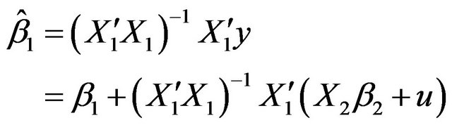
With the above model we now consider the two estimators of β1
1)  from
from 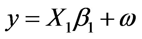 where
where 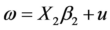
2)  from
from  i.e.
i.e.
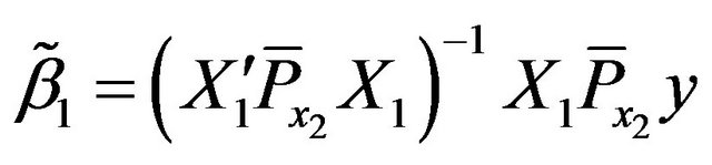 where
where ![]()
With the assumption on  we have immediately that
and since 
This implies 
And 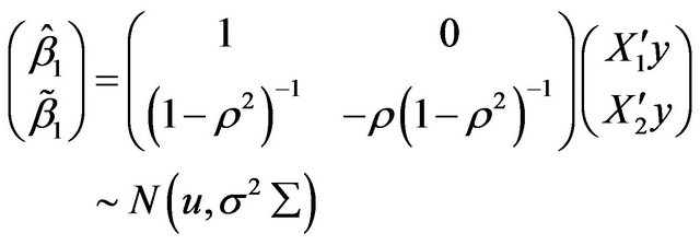
Where 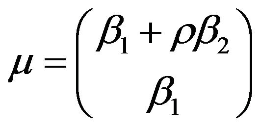 and
and 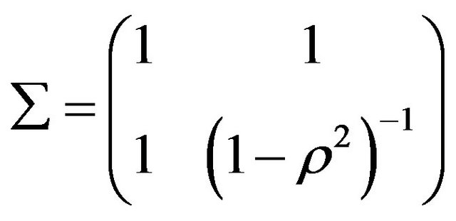
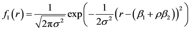
We now calculate the following probability illustrated in the following diagram Figure 1, where the horizontal axis gives values of  while the vertical gives values of
 .
.
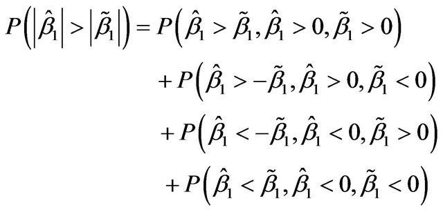
The result is stated in the following Theorem.
Theorem
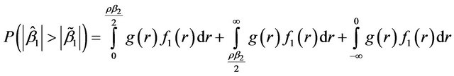
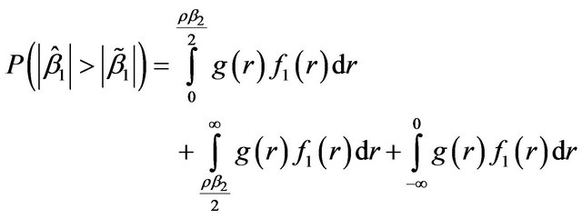
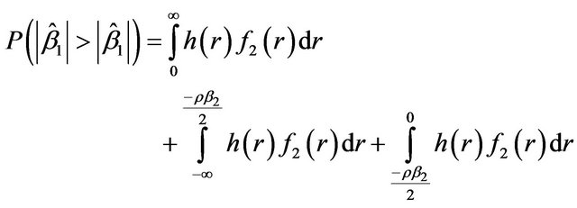
Under the SVSM estimation procedure we have the following probability:
When ρ > 0
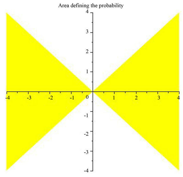
Figure 1. Area defining the probability.
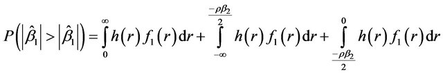
For ρ < 0
where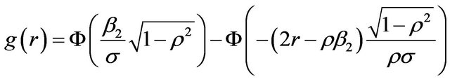 ,
, 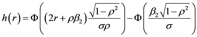
 and
and 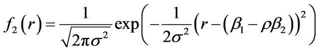
Proof: See Appendix
3. Statistical Analysis
To illustrate our calculations, we carried out some numerical calculations; we calculated the probability that  exceeds
  for different values of σ and ρ; we also computed the R2 of the regression. The values of σ were 0.1, 0.2, 0.5, 1.0, and 2.0 whilst the values of ρ were −0.8, −0.5, −0.2, 0.2, 0.5 and 0.8. Different combinations of
 and
and were used, namely (0.8, 0.4), (0.5, 0.4), (0.4, 0.4), (0.3, 0.4), and (0.1, 0.4). The output constitutes Tables 1-5.
Table 1. Probability and R-squared for  and
and ; (a) Probability for
  and
and ; (b) R-squared for
  and
and .
.
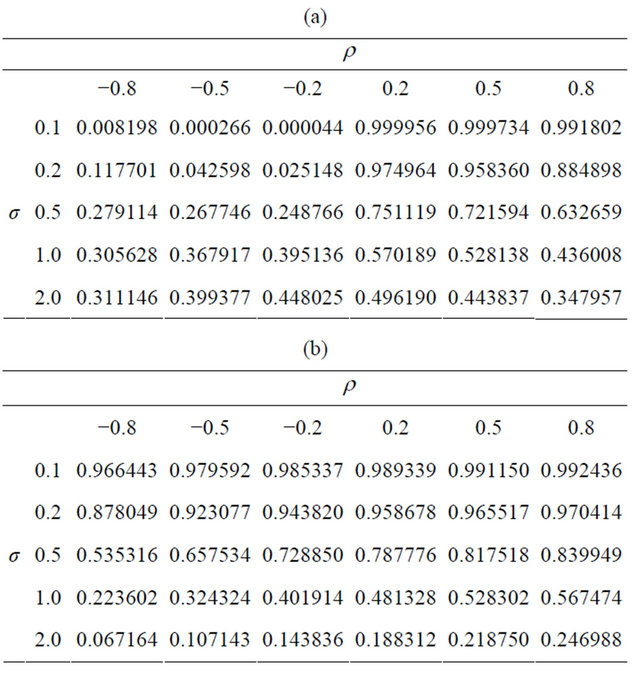
The results show that if the regression was a high R2 and if the two variables are positively correlated, then this procedure leads to a high probability that  exceeds
  not just when
  exceeds
 , but even when
  is less than
  (see Tables 3-5). In the case when R2 is low or when the returns are negatively correlated, the methodology is less successful.
4. Empirical Examples
For illustrative purposes, we use six Fama-French style based portfolios formed on size and book-to-market1. These are: Small Growth (SG), Small Neutral (SN), Small Value (SV), Big Growth (BG), Big Neutral (BN), Big Value (BV). There are two return factors, the first, SMB (Small Minus Big) is the return difference between the average of three small portfolios and the average of three large portfolios, Likewise, the second factor, HML (High Minus Low) is the return difference between the average of two value portfolios and the average of two growth portfolios.
We choose two different sample periods, where SMB and HML are either positively or negatively correlated. Table 6 lists the regression results for the period from 1935 Jan to 1954 Dec, where SMB and HML are positively correlated with ρ = 0.529; Table 7 lists the regression results for the period from 1992 Jan to 2011 Dec with ρ = −0.348. In our sequential variable selection model, SMB is variable 1 and HML is variable 2.  is the estimated coefficient from the univariate regression
Table 2. Probability and R-squared for  and
and ; (a) Probability for
 and
and  (b) R-squared for
  and
and .
.
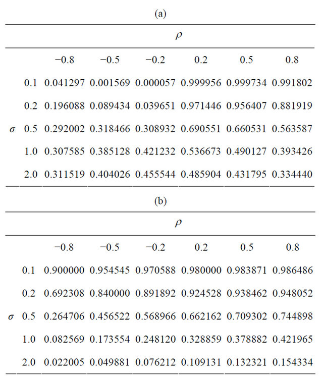
Table 3. Probability and R-squared for  and
and ; (a) Probability for
 and
and ; (b) R-squared for
  and
and .
.
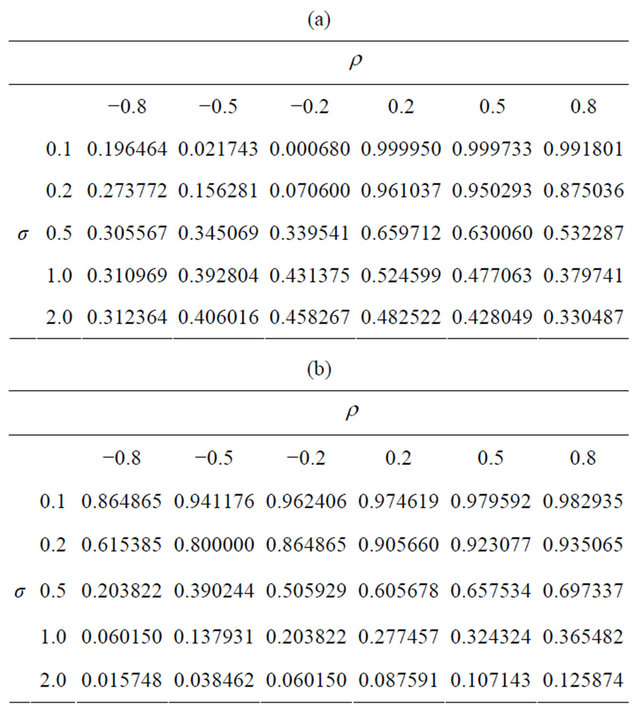
Table 4. Probability and R-squared for  and
and ; (a) Probability for
 and
and ; (b) R-squared for
  and
and .
.
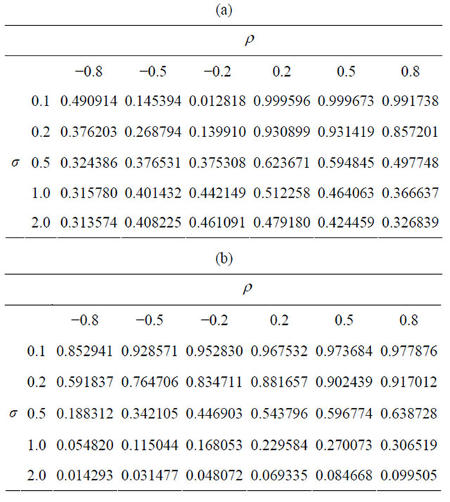
Table 5. Probability and R-squared for  and
and ; (a) Probability for
 and
and ; (b) R-squared for
  and
and .
.
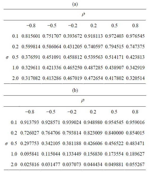
Table 6. Regression results for six portfolios when ρ = 0.529.
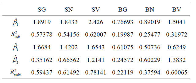
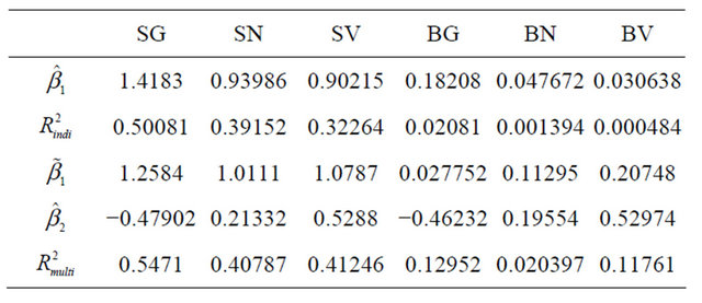
Table 7. Regression results for six portfolios when ρ = −0.348.
of y on SMB;  is the coefficient on SMB from the multiple regression of y on SMB and HML;
  is the coefficient on HML and calculated by regressing the residual of y on SMB upon the residual of HML on SMB.
We are interested in the following question. Under what circumstances will there be a larger estimated exposure  than
than ? The results show that when the two variables are positively correlated as in Table 6, this procedure always generates higher
  than
than . When the two variables are negatively correlated as in Table 7, we identify higher
  than
than  only for two portfolios SG and BG; for the other four portfolios,
  is lower than
 . Therefore comparing the two different cases, we find out that the methodology is more successful when ρ is positively correlated. This confirms our finding in section 3.
5. Conclusions
Bayesian methods are notoriously difficult to implement and practitioners often use tricks to allow their models to reflect their beliefs. We discuss such a procedure, and show analytically conditions when it will work. The particular procedure we discuss is used by practitioners to build factor models. We are interested in the variable selection methodologies that are used to give a particular returns model a particular style and nature. For example, in the context of global models one may wish the model to depend more/less upon domestic factors such as country indices rather than, say, global factors such as currency or world equity/bond markets. The method we discuss allows for favorable selection of a variable by specifying the order in which variables enter a regression.
We strip the problem down to its bare essentials by considering bivariate situations. We evaluate these conditions using numerical integration and further confirm their relevance by looking at an empirical example. The examples used US equity data over 20 years period. These illustrate the efficacy of the procedure.
REFERENCES
- P. Jorion, “Bayes-Stein Estimation for Portfolio Analysis,” Journal of Financial and Quantitative Analysis, Vol. 21, No. 3, 1986, pp. 279-292. doi:10.2307/2331042
- F. Black and R. Litterman, “Global Asset Allocation with Equities, Bonds and Currencies,” Goldman Sachs and Co., New York, 1991. https://faculty.fuqua.duke.edu/~charvey/Teaching/BA453_2006/Black_Litterman_GAA_1991.pdf
- F. Black, and R. Litterman, “Global Portfolio Optimization,” Financial Analysts Journal, Vol. 48, No. 5, 1992, pp. 28-43. doi:10.2469/faj.v48.n5.28
- S. Satchell and A. Scowcroft, “A Demystification of the Black-Litterman Model: Managing Quantitative and Traditional Portfolio Construction,” Journal of Asset Management, Vol. 1, No. 2, 2000, pp. 138-150. doi:10.1057/palgrave.jam.2240011
- A. Gelman, J. Carlin, H. Stern and D. Rubin, “Bayesian Data Analysis,” 2nd Edition, Chapter 5, Chapman & Hall/ CRC, London, 2004.
Appendix: Proof of Theorem
Diagrammatically we need to calculate the two areas in Figure 1 on either side of the origin.
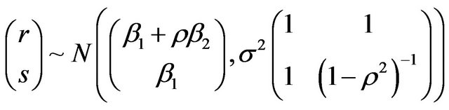
Now
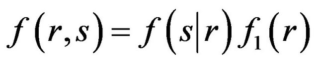
where
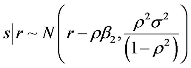
and 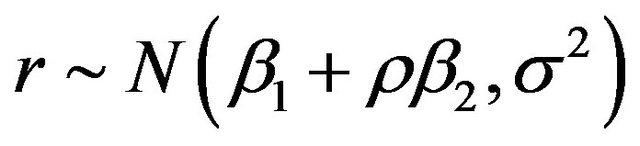
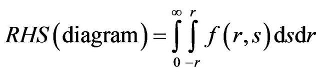
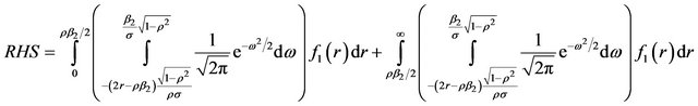
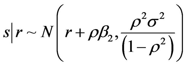
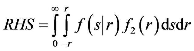
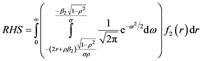
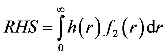
First we shall calculate RHS.
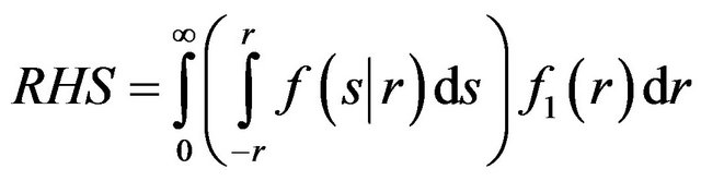
Transforming from s to ω, 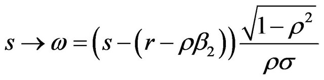
we have 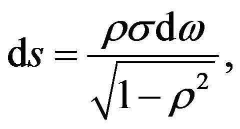 giving
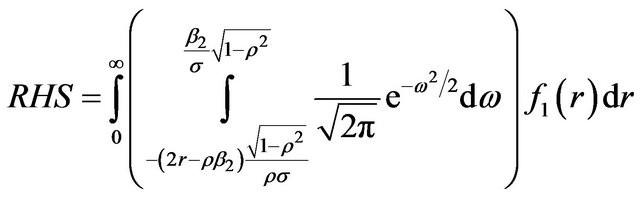
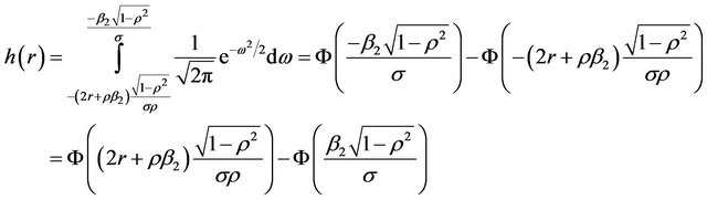
For
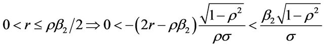
Letting 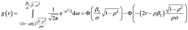
where is the cumulative distribution function of the standard normal distribution we have:
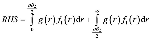
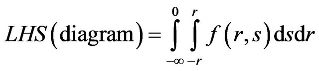
Having completed the calculation of RHS, we now turn to LHS.
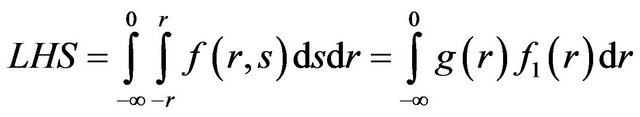
We can make further simplifications depending upon the sign of ρ.
For ρ > 0
where

When ρ< 0 rewrite using –ρ and then let ρ > 0. Thus we now have:
Now,
and again transforming from s to ω, 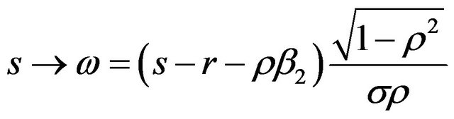 with
with 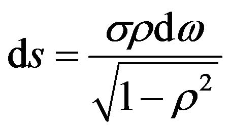
Letting
For 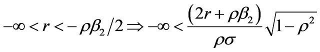
and

Thus for ρ < 0.
where
 .
.
NOTES
1The stocks are ranked based on two independent criteria: size (market capitalization) and book-to-price (the ratio of book value to market value). The median NYSE market equity is chosen to divide the stocks into two groups: big and small; the 30th and 70th percentiles of bookto-price ratio are used to split the stocks into three groups: growth, neutral and value. Six portfolios are formed from the intersection of these independent sorts. Six portfolios are formed from the intersection of these independent sorts.