Journal of Mathematical Finance
Vol.3 No.2(2013), Article ID:31837,11 pages DOI:10.4236/jmf.2013.32031
Recent Developments in Fuzzy Sets Approach in Option Pricing
1Department of Supply Chain Management, University of Manitoba, Winnipeg, Canada
2Department of Statistics, University of Manitoba, Winnipeg, Canada
Email: *appadoo@cc.umanitoba.ca
Copyright © 2013 Srimantoorao S. Appadoo, Aerambamoorthy Thavaneswaran. This is an open access article distributed under the Creative Commons Attribution License, which permits unrestricted use, distribution, and reproduction in any medium, provided the original work is properly cited.
Received January 24, 2013; revised February 27, 2013; accepted March 21, 2013
Keywords: Membership Function; Fuzzy Coefficient; Black-Scholes Partial Differential Equations (PDE); Asset-or-Nothing Option; Fuzzy Real Options
ABSTRACT
Recently there has been growing interest in fuzzy option pricing. Carlsson and Fuller [1] were the first to study the fuzzy real options and Thavaneswaran et al. [2] demonstrated the superiority of the fuzzy forecasts and then derived the membership function for the European call price by fuzzifying the interest rate, volatility and the initial value of the stock price. In this paper, we discuss recent developments in fuzzy option pricing based on Black-Scholes models. Fuzzy coefficient Black-Scholes partial differential equations (PDE) are derived. Membership function of the call price is given. The asset-or-nothing option by fuzzifying the maturity value of the stock price using adaptive fuzzy numbers is also discussed in some detail.
1. Introduction
Most stochastic models involve uncertainty arising mainly from lack of knowledge or from inherent vagueness. Traditionally those stochastic models are solved using probability theory and fuzzy set theory. There exist many practical situations where both types of uncertainties are present. For example, if the price of an option depends upon the nature of the volatility which changes randomly, then the volatility of the stock price movement which is estimated from the sample data is a random variable as well as a fuzzy number. Recently there has been a growing interest in using fuzzy numbers to deal with impreciseness (see Appadoo et al. [3] and Thavaneswaran et al. [4] for more details). Many authors have tried to deal fuzziness along with randomness in option pricing models. For example, recently, Cherubini [5] determined the price of a corporate debt contract and provided a fuzzified version of the Black and Scholes model by means of a special class of fuzzy measures. On the other hand, Ghaziri et al. [6] introduced artificial intelligence approach to price the options, using neural networks and fuzzy logic. They compare the result of artificial intelligence approach to that of Black-Scholes model, using stock indexes. Since the Black-Scholes option pricing formula is only approximate, which leads to considerable errors, Trenev [7] obtained a refine formula for pricing options. Due to the fluctuation of financial market from time to time, some of the input parameters in the Black-Scholes formula cannot always be expected in the precise sense. As a result, Thavaneswaran et al. [4] applied fuzzy approach to the Black-Scholes formula. Zmeskal [8] applied Black-Scholes methodology of appraising equity of a European call option by using the input data in a form of fuzzy numbers. Carlsson and Fuller [9] use possibility theory to study fuzzy real option valuation. Applications of fuzzy sets theory to volatility models have been studied by Thavaneswaran et al. [2] and Thiagarajah et al. [10]. Weidong et al. [11] discuss the analytical solutions for a European option using a fuzzy normal jump-diffusion model and possibility theory. Shiu and Shu [12] propose a fuzzy approach for investment project valuation in uncertain environments from the aspect of real options. Guerra et al. [13] consider the Black and Scholes option pricing model, and present a sensitivity analysis based on the study of the option price when the parameters are supposed to be fuzzy numbers. Zdenek [8] proposed a generalized hybrid fuzzy-stochastic binomial American real option model under fuzzy numbers and Decomposition principle where the Input data are in a form of fuzzy numbers. Xu et al. [14] discuss three different versions of the GarmanKohlhagen model, the put-call parity relationship and the calculation formulas of the Greek letters according to these three different G-K models based on fuzzy set theory. The empirical results indicate that the Greeks calculated under fuzzy environment is a useful tool for managing option risk for an option writer. Nowak and Romaniuk [15] propose the method for option pricing based on application of stochastic analysis and theory of fuzzy numbers. The process of underlying asset trajectory belongs to a subclass of Levy processes with jumps. Thiagarajah et al. [10] present the Black-Scholes option pricing formula with quadratic adaptive fuzzy numbers, their approach hinges on a characterization of imprecision by means of fuzzy set theory.
1.1. Black-Scholes Model
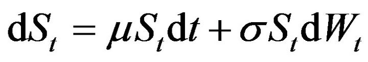
The famous formula of Black-Scholes for the fair prices of European options follows from several assumptions, which are discussed in Metron [16]. Asset prices  are assumed to follow geometric Brownian motion and represented by the equation
 (1.1)
(1.1)
where the process  is a standard Brownian motion,
  is the drift and
  is the volatility of the underlying stock. Generally, a call (put) option is the right to buy (sell) a particular asset for a specified amount at the strike price K at a specified time in the future with the expiration time T. If the option is of such a type that it can be exercised only on the expiration date itself, then it is called a European option. Let
  be the price of the underlying asset at expiration time T. Then the payoff, g, of a European style call option at time T is given by
 (1.2)
(1.2)
This means that the call option is exercised if  and is abandoned otherwise. The above mentioned call and put options are sometimes called plain vanilla or standard options. Let
  be the risk-free interest rate. Then a probability measure
  is called an equivalent martingale measure to the probability measure
  for the discounted price process
  if
if
 (1.3)
(1.3)
for each  and
and , where
  is the history of the process up to time
 . This is the discounted price process
  which is a martingale under the probability measure
 . According to the Fundamental Theorem of Asset Pricing, an arbitrage-free price
  of an option at time
  is given by the conditional expectation of the discounted payoff under an equivalent martingale measure
 ,
,
 (1.4)
(1.4)
Together with this equivalent martingale approach one needs a so-called equivalent portfolio (a combination of other traded assets). Then the price of the option has to coincide with the price of the corresponding equivalent portfolio. Following the results of Black-Scholes, we take a geometric Brownian motion as a stochastic process for modeling the stock price. This model is based on the assumption that the log-returns
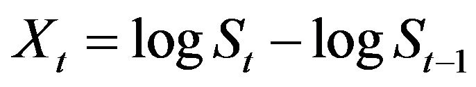 (1.5)
(1.5)
are normally distributed. Now Equation (1.1) becomes
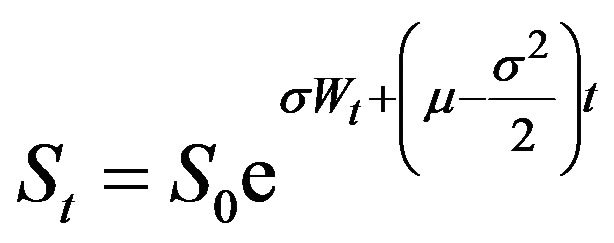 (1.6)
(1.6)
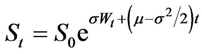
 . Using Itos lemma the model can equivalently be described as
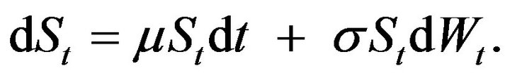 (1.7)
(1.7)
For this model, there exists a unique martingale measure  which is given by Girsanov’s theorem
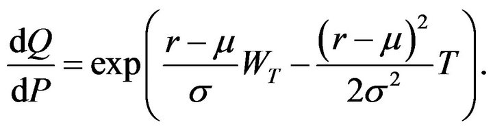 (1.8)
(1.8)
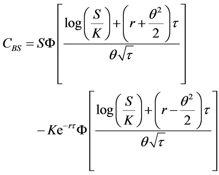
Some calculations yield the Black-Scholes formula as,
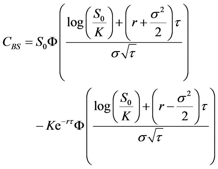 (1.9)
(1.9)
where  denotes the cumulative distribution function of a standard normal variable, and
  denotes the time to expiration. In the literature two different ways of calculating volatility have been discussed. The first method is the empirical estimation from the historical data. The second is to calculate the implied volatility by equating the theoretical call price from the Black-Scholes formula with the market price.
As a benchmark for our analysis we study the standard Black-Scholes [17] option pricing model. We assume that the expiry date and exercise price are always known and non-fuzzy. An interest rate is the amount of money a borrower is obligated to pay the lender. As such, interest rates are differentiated by maturity and default risk of the loan. It is natural to take the rates on Treasury Bills and Treasury bonds, the government securities considered essentially default-free, as natural proxy for a risk-free discount rate for option payoffs. Yet, in practice, overthe-counter derivative traders consider LIBOR rates rather than the government rates as the appropriate cost of capital. LIBOR stands for London Interbank Offer Rate, an interest rate quote by a large bank at which it offers large short-term deposits to other banks. A corresponding bid rate, the rate at which banks accept deposits, is called LIBID. The difference between the sale (ask) and the buy (bid) prices for deposits is analogous to bid-ask spreads in the dealer markets for other securities, e.g., stocks. The existence of the bid-ask spread implies that the true market price is unknown. The bid-ask spread is considered a natural band to represent the uncertainty around the market price. In most empirical work, market prices, either for borrowing/lending or share purchases, are approximated by the mid-point of the bid-ask spread. This procedure among other things introduces errors into model-implied option prices. Another issue is the nonsynchronous record of an option price and the price of the underlying asset. To top it off, true options themselves are traded at bid/ask prices. Using models that do not specifically account for these issues introduces errors-difference between theoretical and observed option premiums. Thavaneswaran et al. [2] modelled the uncertainty of interest rate and stock price using fuzzy numbers.
The rest of this paper is organized as follows. In Section 2, we study the Black-Scholes partial differential equations. Section 3 discusses the asset or nothing option. Section 4 closes the paper with conclusions.
1.2. Preliminaries and Notation
Before discussing the possibilistic moment generating function, we introduce some definitions and properties about fuzzy sets theory with relevant operations.
Definition 1.1 A fuzzy set  in
in , where
  is the set of real numbers, is a set of ordered pairs
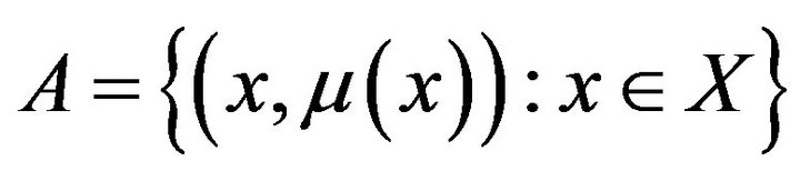 , where
  is the membership function or grade of membership, or degree of compatibility or degree of truth of
  which maps
  on the real interval [0,1].
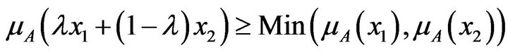
Definition 1.2 A fuzzy set  in
in  is said to be a convex fuzzy set if its
  -level set
  are (crisp) convex sets for all
 . Alternatively, a fuzzy set
  in
in  is a convex fuzzy set if and only if for all
  and
and ,
,
Definition 1.3 A fuzzy number  is called a trapezoidal fuzzy number (Tr.F.N.) with core
 , left width
  and right width
  if its membership function has the following form (see Figure 1 for detail):
 (1.10)
and we use the notation . It can easily be shown that
 (1.11)
The support of  is
is . Moreover, for any fuzzy number
  and a positive real number
 , where the following relationship holds
 . (1.12)
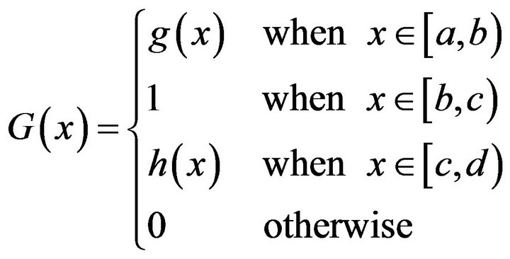
Definition 1.4 Let  be the set of all real numbers. A fuzzy number
 , is of the form
 (1.13)
where g is a real valued, increasing and right continuous function, h is a real valued, decreasing and left continuous function, and  are real numbers such that
 . A fuzzy number A with shape functions g and h defined by
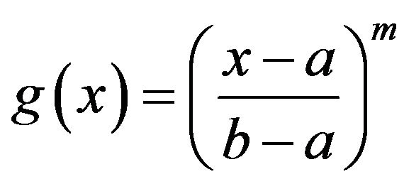 (1.14)
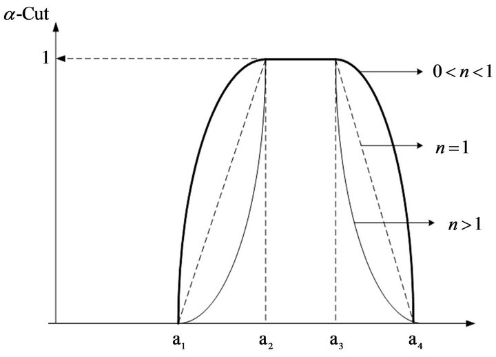
Figure 1. Nonlinear membership function.
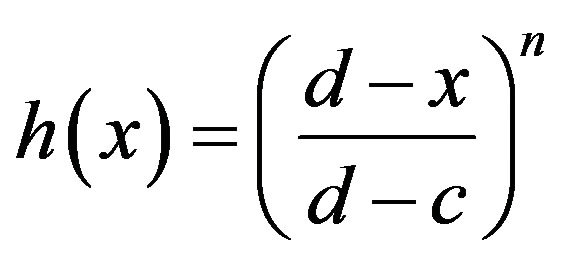 (1.15)
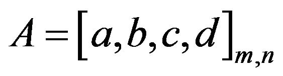
respectively, where m or , will be denoted by
 . If
. If  and
and , we simply write
 , which is known as a trapezoidal fuzzy number. If
  or
or , a fuzzy number
  is a modification of a trapezoidal fuzzy number
 . If
. If  and
and , then
  is a concentration of A. Concentration of A by m and
  is often interpreted as the linguistic hedge “very”. If
 , then
  is a dilation of A. Dilation of A by
  and
and  is often interpreted as the linguistic hedge “more or less”. Each fuzzy number A described by (1.14) and (1.15) has the following
  - level sets (
 -level sets),
 ,
,  ,
,  and
and
If  then, for all
 ,
,
 . (1.16)
1.3. Weighted Possibilistic Moments (WPM)
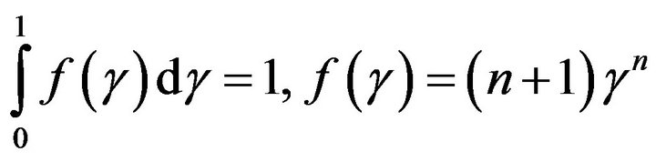
In this section following Carlsson and Fuller [1], we introduce the following moments. The first order f-WPM (or weighted possibilistic mean) of  is given by
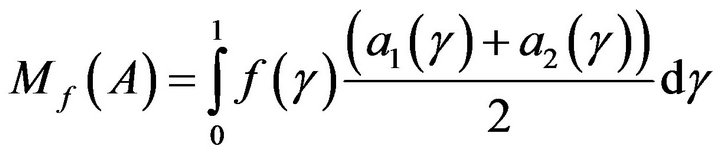 (1.17)
where  is a weight function such that
 .
.
Similarly, the centered WPM (or weighted variance) of  is
is
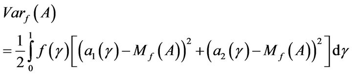 (1.18)
and for any positive integer r, the f-WPM of order r about the possibilistic mean value of A is defined as
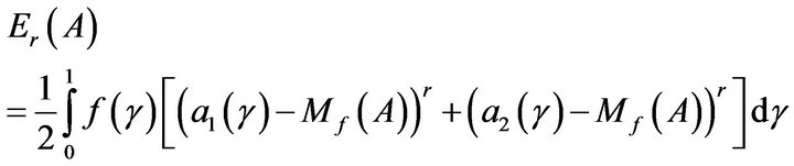 (1.19)
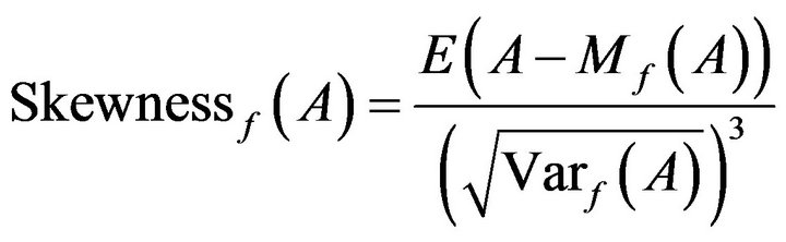
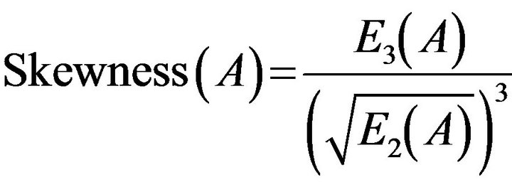
In analogy with Thavaneswaran et al. [4], the fWeighted possibilistic skewness and the f-Weighted possibilistic kurtosis of a fuzzy number A are defined as
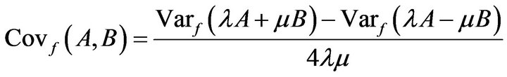
and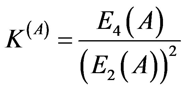 . The f-Weighted possibilistic covariance between two fuzzy numbers A and B is given by
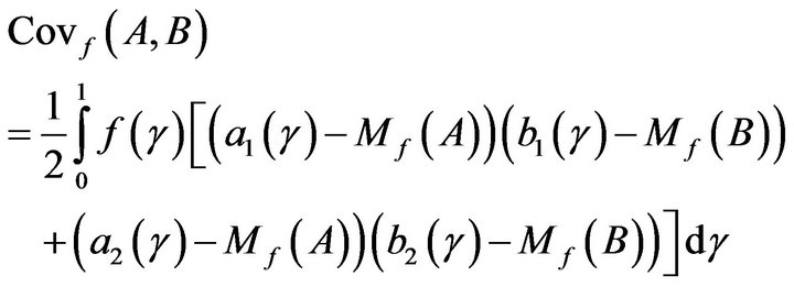 (1.20)
where  is a weight function such that
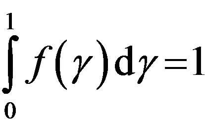 .
.
In analogy with Thavaneswaran et al. [4], the f-Weighted possibilistic skewness of fuzzy number A is defined as
 and similarly, the f-Weighted possibilistic kurtosis of A is defined as
 . If
. If  is an increasing function the
  level sets is given by
 . Now,
 (1.21)
On the other hand if  is a decreasing function the
  -level sets is given by
 . Now,
 (1.22)
Theorem 1.1 Let A and B be two fuzzy numbers and  and
and  positive numbers. Then, we have the following results 1)
2) 

3) 

4) .
.
Let A be a fuzzy number whose  -cuts are given by
  for
for , then the zero centered weighted possibilistic moment generating function is defined as
  if exists
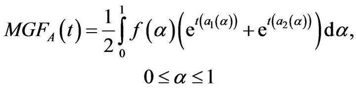 (1.23)
2. Fuzzy Coefficient Black-Scholes PDE
Consider the stock and bond model given by
and
where all of the model coefficients ,
,  , and
, and  are given by explicit function (possibly fuzzy estimates) of the current time and current stock price. Then the arbitrage price at time t of a European option with terminal time T and payout
  is given by
  where
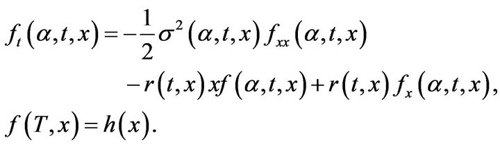
where  is the solution of the PDE
 and its derivatives may be used to provide explicit formulas for the portfolio weights
  and
and  for the self-financing condition portfolio
  that replicates
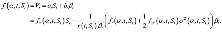
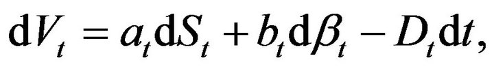
From the self-financing condition and the models for the stock and bond, we have
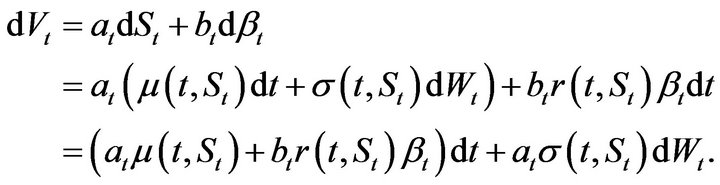
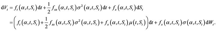
From our assumption that  and the
  formula
The size of the stock portion of our replicating portfolio is:

The  terms cancel, and the bond portion
  is
is
Because  is equal to both
  and
and , the values for
  and
and  give us a PDE for
 :
:
Now, when we cancel  from the last term and replace
  by
by , we arrive at the general Black-Scholes PDE and its terminal boundary condition. The portfolio weights
  and
and  for the self-financing portfolio
  that replicates
  are explicitly given above. Moreover the same argument holds when we use fuzzy estimates for the unknown volatility parameter in the model.
2.1. Fuzzy Coefficient Black-Sholes PDE with Dividends
Suppose that the stock pays a dividend  which is a function of the stock price
 .
.
and
respectively, with the terminal boundary condition
 for all
 .
.
Using cm argument, we arrive at the Black-Scholes PDE:
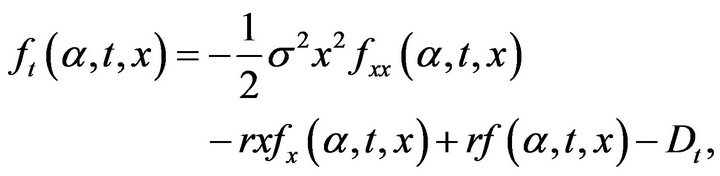
with its terminal boundary condition
 for all
 .
.
2.2. Membership Functions of Call Price
For the Black Scholes model of the form
For this model, there exists a unique martingale measure Q which is given by Girsanov’s theorem
Solving the Black-Scholes PDE, the arbitrage price of the European call option at time  with current stock price S
where  denotes the cumulative distribution function of a standard normal variable,
  is the strike price,
  is the expiry date and
  is the residual time. The amount of stock
  that we hold in the replicating portfolio at time
  is
is
We replace the fuzzy interest rate, the fuzzy stock price, and the fuzzy volatility by possibilistic mean value in the fuzzy Black-Scholes formula. The initial stock price cannot be characterized by a single number. Thus, we assume that the initial stock price is a fuzzy number of the form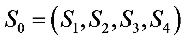 . A fuzzy number of the form
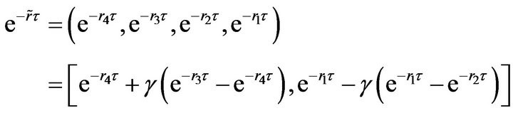
for the discounting factor in a fuzzy sense and of the form 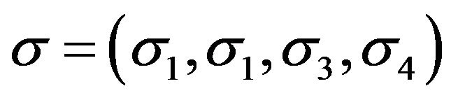 for the volatility can also be modeled in a similar manner. In these circumstances we suggest the use of the following fuzzy weighted possibilistic (heuristic) option formula as in Carlsson and Fuller [9] for computing fuzzy option values. We consider the following Black-Scholes formula for a dividend paying stock with exercise price
 .
.
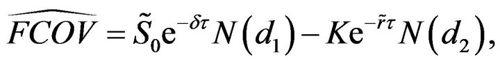 (2.1)
(2.1)
where
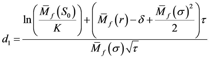 , (2.2)
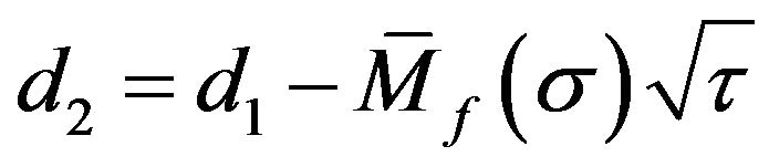 , (2.3)
 is the possibilistic mean value of variable
 . We assume that the stock pays dividends continuously at a known rate
 . The
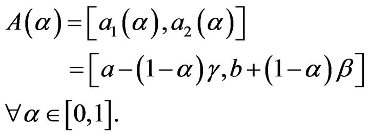
. The  -level sets of the fuzzy call option value
  are as follows:
 (2.4)
(2.4)
where
 (2.5)
(2.5)
 (2.6)
(2.6)
The membership function of the fuzzy call option is given
In the following example we consider the fuzzy call price on a stock option using a fuzzy number discussed earlier.
Example 1 Consider a European call option on a stock with the following assumptions. The current stock price, the stock price volatility and the risk-free interest rate are all taken Tr.F.N fuzzy numbers and
 .
.

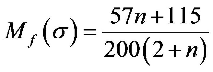
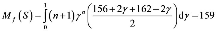
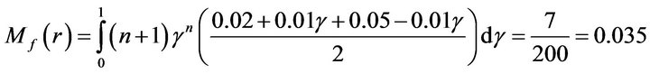
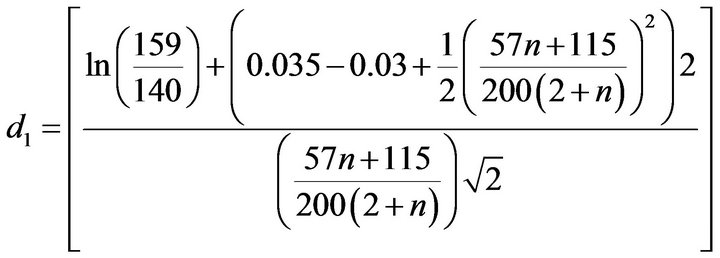
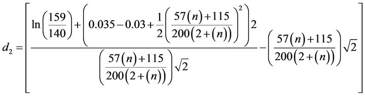
With the help of the above fuzzy expressions we price the call in a fuzzy possibilistic setup.


We present the fuzzy call option values for various levels of  and n as in Table 1 and Figure 2. A fuzzy weighted possibilistic model is sufficiently flexible and can be easily adjusted or tuned for optimal solution. The flexibility is in the ability to choose different values of n according to different criteria. For example, a bank could calibrate n to improve volatility forecasts, which are essential for Value-at-Risk calculations for option portfolios. Alternatively, the value of n can be trained to improve the precision of computed hedge ratios (Greeks).
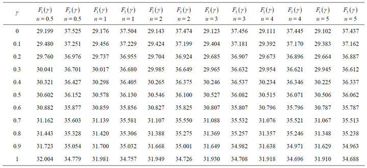
Table 1. The fuzzy call option values for various levels of γ and n.
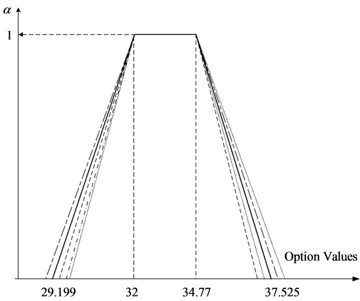
Figure 2. Membership function for different values on n and for 0 ≤ γ ≤ 1.
This may be beneficial for hedging performance, which is essential in risk management.
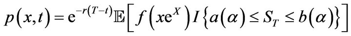
3. General Terminal-Value Claims
A standard option is a contract that gives the holder the right to buy or sell an underlying asset at a specified price on a specified date. The payoff depends on the underlying asset price. The call option gives the holder the right to buy an underlying asset at a strike price; the strike price is termed a specified price or exercise price. Therefore the higher the underlying asset price, the more valuable the call option. If the underlying asset price falls below the strike price, the holder would not exercise the option. Binary option is an exotic call option with discontinuous payoffs. The option pays off a fixed, predetermined amount if the underlying asset price is beyond the strike price on its expiration date. There are two types of binary options: asset-or-nothing call option and cashor-nothing call option. For the first type, the option pays off nothing if the underlying asset price ends up below the strike price. For the second type, the option pays off nothing if the underlying asset price ends up below the strike price and pays a fixed amount if it ends up above the strike price. Note that for the binary option the underlying asset is the stock and the underlying asset price is termed the stock price. The method of pricing the European call option can be used to find the price of any claim in the Black-Scholes model:
 that is
 where
where  and
and  represent the expected return and volatility per unit time, respectively, and
  is a Wiener process. The price at time 0 of a claim paying C at time T is
 , where taking expectations with the martingale probability Q gives the same value as taking expectations with the original probabilities with the assumption that
 ; the price at time t will be
 . Here C may be any
  random variable with
 . The following theorem gives the time t price of a general terminal-value claim
 .
.
Theorem 3.1
1) The time  price of the terminal value claim
  for some real number
  is
is
 2) The time
  price of the asset-or-nothing claim
 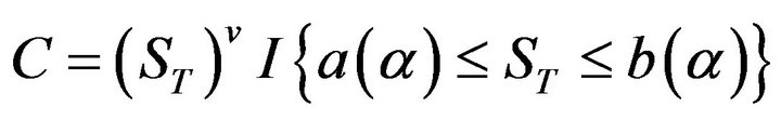 is
is
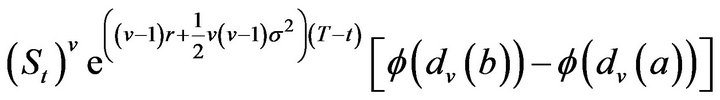 , (3.1)
where
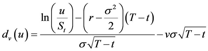 and
and  and
and  are the upper and lower
  - cuts, respectively.
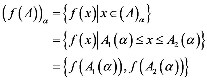
3) For any twice differentiable function  , the time
  price of the terminal value claim
  is given by
where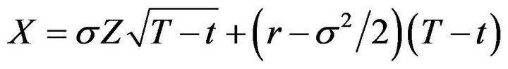 Proof: see A. Thavaneswaran et al. [18].
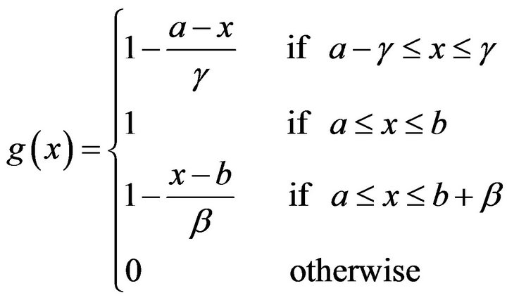
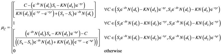
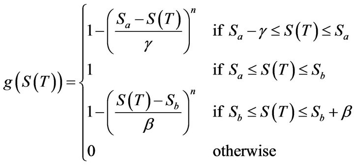
Example 2 For the asset-or-nothing option stated above, the fuzzy concept is taken into account in a model. Define a fuzzy set as trapezoidal fuzzy number with core , left width
  and right width
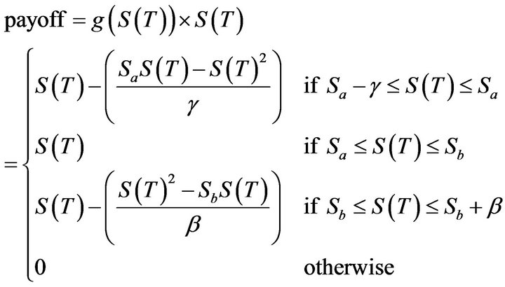
 . Consider the membership function related to asset price which follows the trapezoid function. By introducing the fuzzy concept into a binary function an investor may have more opportunities to think about his decision in some aspect such as risk.
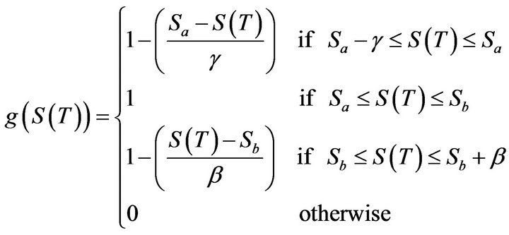 (3.2)
(3.2)
 .
.
The most possible values of the underlying asset price at the maturity date lie in the interval , and
, and 
 is the upward potential and
  is the downward potential for the values of the underlying asset price. For fixing parameter values of
 ,
,  ,
,  , and
, and  there are many ways to be considered. For example, when the investor cannot predict how the underlying asset price changes at the maturity date, in other words, when he becomes confident that the asset price has fluctuated greatly he will take the range of sufficiently large width so that the premium values become high. On the other hand, when much fluctuation is not observed the width will become small, so that
  gets equal to
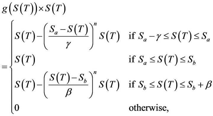
 , resulting in triangular fuzzy numbers. For each of three sets the corresponding payoff is obtained by multiplying its grade of membership function,
 .
.
In this case, and the underlying asset  moves between
  and
and . Then, the present value of option may be computed as a difference between the present value of
  which exceeds
  and that of
  which is above
 .
.
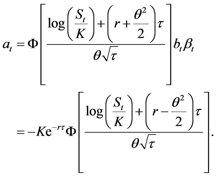
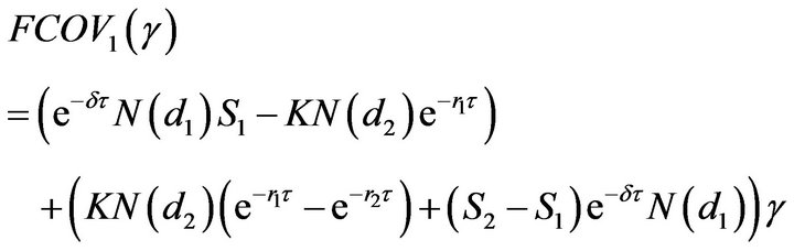
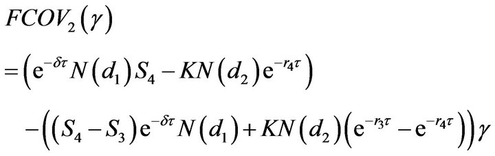
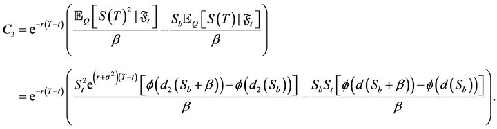
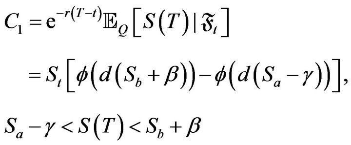
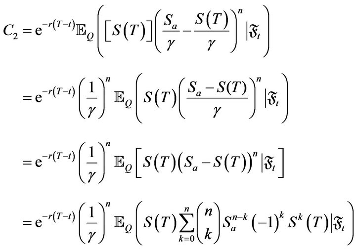
Then, the values of asset-or-nothing option with fuzzy nature are as follows
where
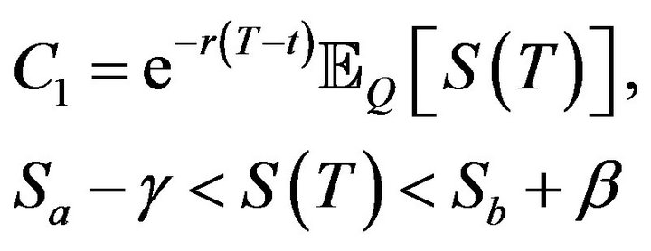
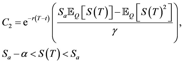
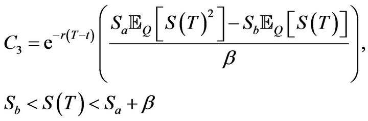
with appropriate boundary conditions, where  denotes the conditional expectation with respect to riskneutral probability.
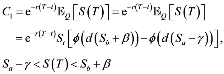
and
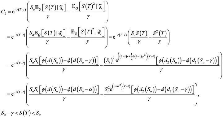
and
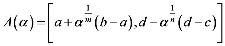
Example 3 When we model the terminal value  by an adaptive fuzzy number having membership function of the form:
 (3.3)
(3.3)
and if the payoff is given by
 (3.4)
(3.4)
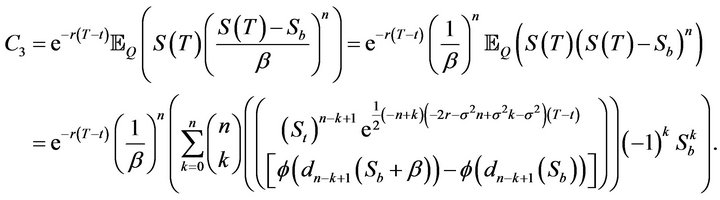
then the time t call price is given by , where
and
It follows from Theorem 3.1,
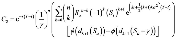
Similarly,
4. Conclusion
In this paper, we have obtained the membership function of the European call price based on the Black Scholes mode with fuzzy volatility. We have fuzzified the maturity value of the stock price using adaptive fuzzy numbers and studied the asset or nothing option. Numerical illustration is given in some detail.
REFERENCES
- C. Carlson and R. Fuller, “On Possibilistic Mean Value and Variance of Fuzzy Numbers,” Fuzzy Sets and Systems, Vol. 122, No. 2, 2001, pp. 315-326. doi:10.1016/S0165-0114(00)00043-9
- A. Thavaneswaran, S. S. Appadoo and A. Paseka, “Weighted Possibilistic Moments of Fuzzy Numbers with Applications to GARCH Modeling and Option Pricing,” Mathematical and Computer Modelling, Vol. 49, No. 1-2, 2009, pp. 352-368. doi:10.1016/j.mcm.2008.07.035
- S. S. Appadoo, “Pricing Financial Derivatives with Fuzzy Algebraic Models: A Theoretical and Computational Approach,” Ph.D. Thesis, University of Manitoba, Winnipeg, 2006.
- A. Thavaneswaran, K. Thiagarajah and S. S. Appadoo, “Fuzzy Coefficient Volatility (FCV) Models With Applications,” Mathematical and Computer Modelling, Vol. 45, No. 7-8, 2007, pp. 777-786. doi:10.1016/j.mcm.2006.07.019
- U. Cherubini, “Fuzzy Measures and Asset Prices: Accounting for Information Ambiguity,” Applied Mathematical Finance, Vol. 4, No. 3, 1997, pp. 135-149. doi:10.1080/135048697334773
- H. Ghaziri, S. Elfakhani and J. Assi, “Neural Networks Approach to Pricing Options,” Neural Network World, Vol. 10, 2000, pp. 271-277.
- N. Trenev, “A Refinement of the Black-Scholes Formula of Pricing Options” Cybernetics and Systems Analysis, Vol. 37, No. 6, 2001, pp. 911-917. doi:10.1023/A:1014542217599
- Z. Zmeskal, “Generalised Soft Binomial American Real Option Pricing Model (Fuzziestochastic Approach),” European Journal of Operational Research, Vol. 207 No. 2, 2010, pp. 1096-1103. doi:10.1016/j.ejor.2010.05.045
- C. Carlsson and R. Fuller, “A Fuzzy Approach to Real Option Valuation,” Fuzzy Sets and Systems, Vol. 139, No. 2, 2003, pp. 297-312. doi:10.1016/S0165-0114(02)00591-2
- K. Thiagarajah and A. Thavaneswaran, “Fuzzy Coefficient Volatility Models with Financial Applications,” Journal of Risk Finance, Vol. 7, No. 5, 2006, pp. 503-524. doi:10.1108/15265940610712669
- X. Weidong, W. Chongfeng, W. J. Xu and H. Y. Li, “A Jump-Diffusion Model for Option Pricing under Fuzzy Environments,” Insurance: Mathematics and Economics, Vol. 44, No. 3, 2004, pp. 337-344.
- S.-H. Hoa and S.-H. Liao, “A Fuzzy Real Option Approach for Investment Project Valuation,” Expert Systems with Applications, Vol. 38, No. 12, 2011, pp. 15296- 15302.
- M. L. Guerra, L. Sorini and L. Stefanini, “Parametrized Fuzzy Numbers for Option Pricing,” IEEE International Conference on Fuzzy Systems, London, 2007, pp. 727- 732.
- W. Xu, W. Xu, H. Li and W. Zhang, “A Study of Greek Letters of Currency Option under Uncertainty Environments,” Mathematical and Computer Modelling, Vol. 51 No. 5-6, 2010, pp. 670-681. doi:10.1016/j.mcm.2009.10.041
- P. Nowak and M. Romaniuk, “Computing Option Price for Levy Process with Fuzzy Parameters,” Vol. 201, No. 16, 2010, pp. 206-210.
- R. C. Merton, “Theory of Rational Option Pricing,” Bell Journal of Economics and Management Science, Vol. 4, No. 1, 1973, pp. 141-183. doi:10.2307/3003143
- F. Black and M. Scholes, “The Valuation of Option Contracts and a Test of Market Efficiency,” Journal of Finance, Vol. 27, No. 2, 1972, pp. 399-417. doi:10.2307/2978484
- A. Thavaneswaran, S. S. Appadoo and J. Frank, “Binary Option Pricing using Fuzzy Numbers,” Applied Mathematics Letters, 2012.
NOTES
*Corresponding author.