Open Journal of Statistics
Vol.09 No.01(2019), Article ID:90564,9 pages
10.4236/ojs.2019.91009
A Note on Improving Inference of Relative Risk
Octavia C. Y. Wong
School of Kinesiology and Health Science, York University, Toronto, Canada

Copyright © 2019 by author(s) and Scientific Research Publishing Inc.
This work is licensed under the Creative Commons Attribution International License (CC BY 4.0).
http://creativecommons.org/licenses/by/4.0/


Received: January 11, 2019; Accepted: February 16, 2019; Published: February 19, 2019
ABSTRACT
Relative risk is a popular measure to compare risk of an outcome in the exposed group to the unexposed group. By applying the delta method and Central Limit Theorem, [1] derives two approximate confidence intervals for the relative risk, and [2] approximates the confidence interval for the relative risk via the likelihood ratio statistic. Both of these approximations require sample size to be large. In this paper, by adjusting the likelihood ratio statistic obtained by [2] , a new method is proposed to obtain the confidence interval for the relative risk. Simulation results showed that the proposed method is extremely accurate even when the sample size is small.
Keywords:
Bartlett Correction, Confidence Intervals, Coverage Property, Relative Risk

1. Introduction
Consider two groups of subjects: exposure group (i = 1) and control group (i = 2). Let ni be the number of subjects in group i with being the risk of a specific outcome in group i. Then the random variable , which is the number of subjects that give the specific outcome in group i, is distributed as Binomial ( , ). As defined in [3] and [4] , the relative risk of the outcome in the exposure group versus the control group is . Note that can be any nonnegative real number. When , it suggests that the exposure being considered is associated with a reduction in risk, and suggests that the exposure is associated with an increase in risk. is generally of interest because it suggests that the exposure has no impact on risk. In general, pi is unknown, but we observed xi. Then pi can be estimated by . And, therefore, an estimate of the relative risk based on the observed sample is .
Relative risk is a popular measure used in biomedical studies because it is easy to compute and interpret, and it is included in standard statistical software output (e.g., in R and SAS). [5] gives a detailed discussion on the application of relative risk to failure time data. [6] applies relative risk to study populations with differing disease prevalence. [7] compares relative risk with odds ratio, and absolute risk reduction in comparing the effectiveness of certain treatments.
To illustrate the concept of relative risk, let us consider the following example. [1] examined the Physicians’ Health Study, which analyzed whether taking aspirin regularly will reduce cardiovascular disease. Data of the study are reported in Table 1.
Out of 11,037 physicians taking aspirin over the course of the study, 104 of them had heart attacks. Similarly 189 of 11,034 physicians in the placebo group had heart attacks. Based on this dataset, the relative risk of having heart attacks among physicians is
Thus, physicians who took aspirin over the course of the study have 0.55 times the risk of having a heart attack as physicians who were in the placebo group. This suggests that taking aspirin is associated with a reduction in the risk of heart attacks among physicians as they are about half as likely to have a heart attack as physicians who did not take aspirin throughout the study.
Although reporting a point estimate of relative risk is important, it does not provide information about the variations arising from the observed data. Hence, in practice, a confidence interval for is usually reported and recommended (see [8] ). A standard approximated confidence interval for is given in [1] , which is widely implemented in statistical software. [2] proposed an alternate way of approximating a confidence interval for via the likelihood ratio statistic. It is well-known that both methods are not accurate when the sample size is small. In this paper, by adjusting the likelihood ratio statistic obtained by [2] , a new method is proposed to obtain the confidence interval for the relative risk. Simulation results show that the proposed method is extremely accurate even when the sample size is small.
2. Methology
Let , i = 1, 2, be independent random variables distributed as Binomial ( , ). Then the relative risk is defined as . A standard estimator of is . With realizations and , a standard estimate of is . [1] considered the parameter . The corresponding estimator of is . By applying the delta method, we have

Table 1. Cross-classification of aspirin use and heart attack.
and
Therefore, an estimate of is , and the estimated variance of is
Hence, when and are large, by the Central Limit Theorem, an approximate confidence interval for is:
where is the percentile of the standard normal distribution. Since and are one-one correspondence, we have an approximate confidence interval for is
The above interval is directly available from R using the riskratio() command.
Since is a biased estimator of , [1] suggests using a modified estimator for , which takes the form
and .
The estimated variance of is
Thus, the corresponding approximate confidence interval for is
.
[2] proposed to construct an approximate confidence interval for based on the likelihood ratio statistic. Since are independently distributed as Binomial ( , ), the joint log-likelihood function is
The point that maximizes the log-likelihood function is known as the maximum likelihood estimate (MLE) of , which can be obtained by solving
and .
In this case, the MLE of is . Moreover, for a given
value, the point that maximized the log-likelihood function subject
to the constraint is known as the constrained MLE of . [2]
gives a numerical algorithm to obtain . However, by applying the Lagrange multiplier technique, we have the explicit closed form of the constrained MLE:
and
The observed likelihood ratio statistic is
.
With the regularity conditions given in [9] , the Wilks Theorem can be applied, and hence, is asymptotically distributed as the chi-square distribution with 1 degree of freedom, . Therefore, the approximate confidence interval for obtained in [2] is
where is the percentile of the distribution.
It is well-known that the above methods are not very accurate when the sample size is small. Although is asymptotically distributed as distribution, except in special cases, , which is the mean of the distribution. [10] proposed a scale transformation of , such that the mean of the transformed statistics is the mean of the distribution. This transformed statistic is known as the Bartlett corrected likelihood ratio statistic. Mathematically, let the Bartlett corrected likelihood ratio statistic be
.
Then is asymptotically distributed as distribution and . However, the explicit form of is only available in a few well-defined problems.
In this paper, I propose to use the following algorithm to approximate and hence the observed Bartlett corrected likelihood ratio statistic .
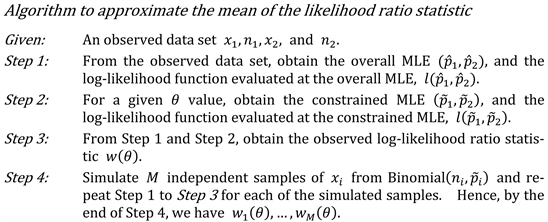
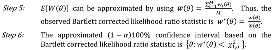
Note that the key step of the algorithm is Step 4 where we simulate new data from the Binomial distribution where the parameter is chosen to be the constrained MLE obtained in Step 2. The reason is that we are trying to obtain a sampling distribution of the likelihood ratio statistic , which is a function of the value given in Step 2. Hence, constrained MLE is used in Step 4.
As a final note in this section, the method by [2] is a computationally intensive method because, to obtain the required confidence limits, we need to find the smallest value and also the largest value such that . The same needs to be done for the proposed method. However, the [1] methods have a closed form expression of the confidence limits, so they are easier to calculate and are available in statistical software.
3. Results
Our first example is to revisit the dataset discussed in previous section. Table 2 recorded the 95% confidence interval for the relative risk obtained by the method discussed in this paper. Since the sample sizes are very large, it is not surprising that all the intervals are very close to each other.
As for our second example, the number of divorces during 2006 in a random sample of Army Reserve and Army Guard couples is reported in [11] . The data are presented in Table 3.
The estimated relative risk is , which indicates that the divorce rate for Army Reserve personnel is higher than the divorce rate of the
Table 2. 95% confidence interval for the relative risk of having heart attacks among physicians taking aspirin versus physicians taking a placebo.
Table 3. The number of divorces during 2006 in a random sample of Army Reserve and Army Guard couples.
Army Guard. Table 4 recorded the 95% confidence interval for the relative risk obtained by the method discussed in this paper. Despite the sample sizes being relatively large, the results are still quite different.
For this example, we also calculated the probability that the true relative risk is as extreme or more extreme than the estimated relative risk by the four methods discussed in this paper. The results are plotted in Figure 1(a) for small true relative risk and Figure 1(b) for large true relative risk. The plots clearly showed that the four methods give different results especially when the true relative risk is large.
Hence, it is important to investigate which method is more accurate when sample size is small. The following simulation studies were performed.
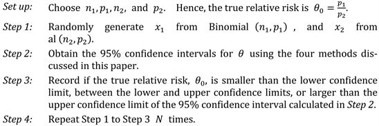
Note that the proportion of samples with less than the lower confidence limit is known as the lower error proportion, the proportion of samples with larger than the upper confidence limit is known as the upper error proportion, and the proportion of samples with falling within the confidence interval is known as the central coverage proportion. Moreover, the average absolute bias is defined as
,
which is a measure of bias of the 95% confidence interval. The nominal values for the lower error proportion, central coverage proportion, upper error proportion, and average absolute bias are 0.025, 0.95, 0.025, and 0, respectively.
Table 5 records the lower error proportion, central coverage proportion, and upper error proportion for a sample of simulation studies that I have performed. Results for other combinations of and are very similar and are available upon request.
Table 4. 95% confidence interval for the relative risk of divorce in the Army Reserve versus the Army Guard.
Table 5. Lower error proportion (le), central coverage proportion (cc), upper error proportion (ue), and absolute average bias (aab) of the 95% confidence interval for θ with N = 10,000 and M = 200.
Note: Method 1 = Agresti’s method without adjustment, Method 2 = Agresti’s method with adjustment, Method 3 = Zhou’s method, and Method 4 = Proposed method.
 (a)
(a) (b)
(b)
Figure 1. (a) and (b) show probability that the true relative risk is as extreme or more extreme than the estimated relative risk.
From Table 5, the two methods by [1] do not give satisfactory results. While one can argue that they have decent central coverage proportion when the sample sizes are large, they also have asymmetric tail errors. Moreover, although the aim of the adjusted method in [1] is a bias adjustment to the standard point estimator, it has little effect on the central coverage proportion, and it has adverse effect on the tail errors proportion. [2] method gives good central coverage proportion, but the tail errors are asymmetric. The proposed method outperformed the other three methods discussed in this paper regardless of the sample sizes.
4. Conclusion
In this paper, we demonstrated via simulations that the two methods discussed in [1] , which are implemented in most standard statistical software, do not have good central coverage properties and the tail errors are extremely asymmetric, particularly when the sample sizes are small. Thus, practitioners should interpret confidence intervals obtained from standard statistical software with caution, especially when the sample sizes are small. The likelihood ratio method proposed in [2] has good central coverage, but the tail errors are asymmetric, which is still an improvement over [1] methods. In comparison, the proposed modification of the likelihood ratio method outperforms the other three methods in terms of both central coverage and tail error symmetry even when the sample sizes are small.
Conflicts of Interest
The author declares no conflicts of interest regarding the publication of this paper.
Cite this paper
Wong, O.C.Y. (2019) A Note on Improving Inference of Relative Risk. Open Journal of Statistics, 9, 100-108. https://doi.org/10.4236/ojs.2019.91009
References
- 1. Agresti, A. (2012) Categorical Data Analysis. 3rd Edition, Wiley, New York.
- 2. Zhou, M. (2018) Confidence Intervals for Relative Risk by Likelihood Ratio Test. Biostatistics and Biometrics Open Access Journal, 6, 1-3. https://doi.org/10.19080/BBOAJ.2018.06.555700
- 3. Sistrom, C.L. and Garvan, C.W. (2004) Proportions, Odds, and Risk. Radiology, 230, 12-19. https://doi.org/10.1148/radiol.2301031028
- 4. Di Lorenzo, L., Coco, V., Forte, F., Trinches, G.F., Forte, A.M. and Pappagallo, M. (2014) The Use of Odds Ratio in the Large Population-Based Studies: Warnings to Readings. Muscles Ligaments and Tendons Journal, 4, 90-92. https://doi.org/10.11138/mltj/2014.4.1.090
- 5. Kalbfleisch, J.D. and Prentice, R.L. (2011) The Statistical Analysis of Failure Time Data. 2nd Edition, Wiley, New York.
- 6. Tenny, S. and Bhimji, S.S. (2017) Relative Risk. StatPearls. https://www.ncbi.nlm.nih.gov/books/NBK430824
- 7. Schechtman, E. (2002) Odds Ratio, Relative Risk, Absolute Risk Reduction, and the Number Needed to Treat—Which of These Should We Use? Value Health, 5, 431-436. https://doi.org/10.1046/J.1524-4733.2002.55150.x
- 8. Gardner, M.J. and Altman, D.G. (1986) Confidence Intervals Rather Than P-Values: Estimation Rather Than Hypothesis Testing. British Medical Journal (Clinical Research Edition), 292, 746-750. https://doi.org/10.1136/bmj.292.6522.746
- 9. Shao, J. (2009) Mathematical Statistics. 2nd Edition, Springer, New York.
- 10. Bartlett, M.S. (1937) Properties of Sufficiency and Statistical Tests. Proceedings of the Royal Society A: Mathematical, Physical and Engineering Sciences, 160, 268-282.
- 11. Kokoska, S. (2011) Introductory Statistics: A Problem-Solving Approach. Freeman, New York.