Open Journal of Statistics
Vol.06 No.05(2016), Article ID:71404,11 pages
10.4236/ojs.2016.65068
Prediction of Civil Aviation Passenger Transportation Based on ARIMA Model
Xinxin Tang1, Guangming Deng1,2
1College of Science, Guilin University of Technology, Guilin, China
2Institute of Applied Statistics, Guilin University of Technology, Guilin, China

Copyright © 2016 by authors and Scientific Research Publishing Inc.
This work is licensed under the Creative Commons Attribution International License (CC BY 4.0).
http://creativecommons.org/licenses/by/4.0/


Received: August 15, 2016; Accepted: October 18, 2016; Published: October 21, 2016
ABSTRACT
The passenger transportation, as an important index to describe the scale of aviation passenger transport, prediction and research, can let us understand the future trend of the aviation passenger transport, according to it, the airline can make corresponding marketing strategy adjustment. Combining with the knowledge of time series let us understand the characteristics of passenger transportation change, the R software is used to fit the data, so as to establish the ARIMA(1,1,8) model to describe the civil aviation passenger transport developing trend in the future and to make reasonable predictions.
Keywords:
Passenger Transportation, ARIMA Model, Seasonal Trend, Forecast

1. Introduction
In recent years, with the improvement of people’s living, travel distance extension, travel mode is no longer confined to the car and train traffic. And taking into account the cost of time, more and more people choose the aircraft as means of transportation to travel. Some scholars have done research on the characteristics of China’s air transport development [1] that with the development of the national economy it has a certain period of regularity. As China’s comprehensive national strength, the aviation market will also have the potential to develop more. Passenger demand forecasting value of civil aviation is the key factor to determine the size of the passenger transport market. This article will focus on the future development of civil aviation passenger transport prospects.
Now prediction methods that have complete theoretical basis mainly include: regression analysis, time series analysis, input-output method, inductive method and Markov chain prediction method. At present, China has already done the research and forecast of aviation passenger traffic. In terms of influence factors, Wang Cui (2008) [2] from the perspective of macroeconomic and microeconomic analysis, found that there are many factors impact the air passenger volume and the factors include non quantifiable factors. Deng Jiejun and Luo Li (2006) [3] , based on the relationship between social economic development and civil aviation passenger demand, use the method of multiple linear regression and GMDH to predict and analyze the demand of civil aviation passenger transport. In methodology, Chen Lihua (2003) [4] , in accordance with the method of regression analysis, taking domestic and international airline passenger turnover as a result of variables, predicts the total turnover of passengers. Wang Xiaoguang et al. (2008) [5] proposed a model which based on artificial neural network and the combination of the polynomial model to forecast the volume of passenger. Pan Ling et al. (2014) [6] established the product season model to forecast the civil aviation passenger traffic volume from December 2013 to December 2014. Kong Jianguo et al. (2014) [7] used the wavelet analysis theory to forecast the demand of civil aviation passenger transport.
Because there are many factors influencing the air passenger volume, we need in-depth study of the internal and external environment of the aviation industry. The influence factors include the non quantifiable factors which are not easy to treatment, so this paper selects the self factor model focuses on its internal rules. In economic forecasting process, the ARIMA model (i.e., autoregressive moving average model) not only considers the economic phenomena in time series dependence, but also considers the interference of random fluctuations. On this problem of short-term trend forecast for the economic operation, this model has the high accuracy rate. The ARIMA model is widely used in economic research. Because of many factors such as holidays and climate factors, the aviation passenger transport industry has the market volatility. The passenger volume can be regarded as a stochastic time series formed with the passage of time. By analysing the time series is stochastic, stationary and seasonal factors or not, we can use the ARIMA model to fit civil aviation passenger transport. Therefore, this paper will use the time series analysis of the ARIMA model and R software to fit the data to achieve passenger transport turnover forecast. Air passenger traffic turnover is a composite index that can describe air transport enterprises in a certain period of time. It is a composite index of transport volume and distance. Air passenger traffic turnover is not only an important index of civil aviation enterprises, but also one of the main indicators of the national assessment of air transport enterprises. Therefore, this paper will study the problem of air passenger transport turnover forecast.
2. Theoretical Basis
2.1. ARIMA Model
In the domestic and foreign well-known materials or works, modeling method of time series is basically uniform that the steady but autocorrelation sequence to establish ARMA model and the non-stationary time series (with unit root) to establish ARIMA(p,d,q) model [8] .
The ARIMA(p,d,q) model includes the autoregressive model AR(p), moving average model MA(q) and the mixed autoregressive moving average model ARMA(p,q) of these three cases [9] .
The first one, the AR(p) model corresponding to the algebraic expression is:
 (1)
(1)
The second, the MA(q) model of the corresponding algebraic expression is:
 (2)
(2)
Third, the ARMA(p,q) model corresponds to the logarithmic expression is:
 (3)
(3)
If  is not smooth, but
  is smooth, then integrating the ARMA model to be ARIMA(p,d,q) for the use of a smooth process
  to replace the position of the unstable
  in the ARMA model.
Among them, both  and
and  are the parameters to be estimated and L is the lag operator.
2.2. STL Decomposition Method
The STL [10] is a time series decomposition method with robust local weighted regression as the smoothing method. And the Loess method is a local polynomial regression fitting, which is a common method for smoothing the two dimensional scatter points. It combines the simplicity of the traditional linear regression and the flexibility of the nonlinear regression. When you want to estimate a response variable value, it is first to get a subset of data from the forecast variables nearby, then use linear regression or quadratic regression on the subset regression. The weighted least squares method is adopted, which is close to the estimated value of the point of greater weight. Finally, using the local regression model to estimate the value of the response variable. The whole fitting curve is obtained by the method of point by point operation. This method has a lot of advantages. For example, it can handle any type of seasonal data, the quarter component can be allowed to change over time, it can control the rate of change, and has better robustness to outliers. The disadvantage of this method is that it is only applicable to the additive model.
The STL decomposition method corresponds to the logarithmic expression is:
 (4)
(4)
Among them,  as the raw data,
  is the trend of low pass filtering of time series data,
  indicates trend smoothing and
  is the final result obtained by the STL decomposition method.
3. Source and Pretreatment of Data
This article studies on the index (civil aviation passenger transport volume [11] ) data from the main indicators of transportation and production, which be downloaded from the Civil Aviation Administration of China. This paper studies the data for the monthly data from January 2010 to August 2015. Through the R software to draw the timing diagram, as shown in Figure 1.
It can be seen from Figure 1 that the passenger turnover has a strong seasonal cycle, in August each year to reach a significant peak and February is trough. And it can be seen that the turnover of passenger traffic has been increasing in accordance with a relatively stable trend year by year.
The change of seasons can make the time series of passenger turnover change regularly, which is the seasonal periodicity seen in Figure 1. There are many reasons for the seasonal changes, such as climate, holidays and so on. Through seasonal adjustment which can eliminate seasonal effects in the sequence, it to be able to more clearly reveal the trend of the time series [12] . In order to reflect the essential attribute of the objective economy more accurately, we need to take some methods to eliminate and adjust the seasonal variation factors in time series.
From January 2010 to August 2015 passenger turnover data into R software, based on the Loess method to do seasonal trend decomposition. This trend decomposition method is STL decomposition method, which is a time series decomposition method with generality and robustness. Thus it gets the seasonal trend decomposition map (it is shown in Figure 2).

Figure 1. Chinese civil aviation passenger transportation time sequence diagram.

Figure 2. Seasonal trend decomposition.

Table 1. Seasonal variation of each month.
As can be seen from Figure 2, the data is divided into three parts, the trend, season and redundancy, in which the various parts of the seasonal variation of the specific data as shown in Table 1. The upward curve of the top of Figure 2 is the development trend of passenger turnover, and the information of the time sequence diagram is consistent with it. Table 1 shows that each year in January is the trough of passenger turnover, in August is the peak of the turnover of passenger traffic.
After understanding the basic trend of the civil aviation passenger transport, in order to effectively predict the future trend of development, we need to fit the passenger transport turnover curve. First, we need to remove the seasonal changes in the time series. And then we make the remaining part of the data for ADF test.
When the ADF level is 0.01, 0.05 and 0.1, the critical value of them is −3.99, −3.45 and −3.13 respectively (the smaller the value of the more significant). And the test results show that the test statistic value of the original sequence is 0.1015, there is no sufficient evidence to reject the original hypothesis. It can not say that the original sequence is smooth. Then after the first order difference of the original data, the test statistic obtained is −5.6418, which is significant at 0.01 level, that is to reject the original hypothesis. Therefore, before the construction of the ARMA model to the data for the first order difference.
4. Construction of Model
Through the R software output the timing diagram of data (it is shown in Figure 3), although it is the removal of seasonal change but still retain most of the sequence information of the original data. The next step is building ARIMA model.
For the ARIMA(p,d,q) model identification, it is required to determine the three parameters of p, d, q. The identification of parameter d has been completed, through the

Figure 3. Remove timing map data seasonally (on), after the first order difference of ACF (lower left) and PACF (lower right).
first order difference, the sequence is smooth. So we think the time series is a single integer sequence and it can construct ARMA model after the first order difference. Under normal circumstances, it can be used for the self correlation function ACF map and the partial autocorrelation map PACF map to initially identify p and q. But it is very difficult to see the order in the ACF diagram and PACF diagram. In this paper, we introduce the concept of Bayesian information criterion. BIC is developed from the Bayesian perspective, which is similar to the maximum probability of a posteriori model, and a priori model has a uniform distribution in all models [13] .
The expression formula of BIC is as follows:
 (5)
(5)
Among them, L is the maximum likelihood, n represents the number of data, K said the number of variables in the model.
The BIC criterion is used to describe the loss of information after using a certain model relative to the actual situation. So the smaller the BIC value indicates that the model fitting effect is better. According to the BIC criterion to judge that for different q and p display the corresponding BIC value, the results shown in Figure 4.
As can be seen from Figure 4, the model that minimizes the value of BIC is ARMA(1,8).
It uses ARMA(1,8) model to fit the data which removed seasonal variation (already through the first order difference) and points out the value of p [14] when the lag for

Figure 4. For different p and q shows the corresponding BIC value.

Figure 5. ARMA fitting with the data residuals of the Ljung-Box test of the p value (on), ACF (lower left) and PACF (lower right).
the Ljung-Box test is 1 - 30, ACF diagram and PACF diagram is shown in Figure 5.
The null hypothesis of Ljung-Box test is that the sequence is independent, for the observed value of p which is not related to should be very large. If the value of p is small that it may be correlated. From Figure 5, we can see that the residual are greater than 0.8, so the residual is white noise and the fitting effect is good. Therefore the model of fitting civil aviation passenger transport turnover is ARIMA(1,1,8), the formula is as follows:
 (6)
(6)
In the upper representation,  is the sequence of the first order difference.
5. Forecast Result and Analysis
According to the fitting results of the sequence, the ARIMA(1,1,8) model of civil aviation passenger turnover has passed the test, and the fitting effect is ideal. It can be used to forecast the change of passenger turnover in the future. Using R software to predict the value of passenger turnover in the next 6 months, it draws a forecast figure as shown in Figure 6.
Figure 6 shows the range of passenger traffic volume prediction within the range of error allowed. On the basis of the predicted value of the air passenger turnover, it adds up to the seasonal variation of each month (see Table 1), that is to get the civil aviation passenger transport turnover from the next six months, as shown in Table 2.
As can be seen from the Table 2, the next six months the amount of air passenger traffic to maintain a rising trend, which is affected by seasonal fluctuations will still fluctuate, but the prospects for the airline passenger market is still very impressive. It is worth mentioning that, with the original data of seasonal variation by the seasonal trend decomposition is different, the volume of passenger transport will occur a slightly lower expected value in November 2015, the passenger turnover may be declined in this
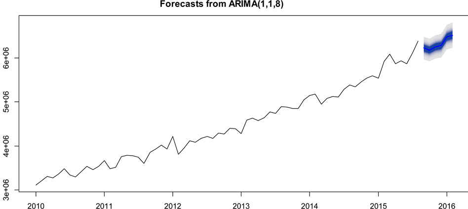
Figure 6. ARIMA(1,1,8) prediction map.
Table 2. Comparison between the predicted and true value of passenger transportation.
period of time, but this does not affect the rising trend of the total passenger traffic volume. After comparing with the real data, the prediction error is maintained at about 1%, and the predicted results are in line with the expected results. Same as the predicted results, there is a lower value in November and the overall trend is still maintained steady growth.
This paper draws a line chart of the passenger turnover amount, as shown in Figure 7. From Figure 7, we can clearly see that the predicted value and the true value is very close, the model has a high prediction accuracy.
6. Conclusions and Recommendations
Time series analysis is performed by the civil aviation monthly passenger volume data from January 2010 to August 2015, this article established the ARIMA(1,1,8) model. On the basis of the ARIMA model to predict the trend of passenger turnover from next 6 months, the fitting effect of this model is better. The following conclusions are obtained by the ARIMA model of passenger turnover:
First, as China’s comprehensive national strength and people’s living standards to be better, air passenger volume will maintain a steady upward trend, it will officially break the mark of 6 ten thousand person-kilometers. And air passenger market will become bigger.
Second, the passenger turnover has a certain seasonal fluctuation, the main reasons of which include holidays, climate and so on. For example, summer (that is August) is

Figure 7. Comparison between the predicted and true value of passenger transportation.
the peak of the air passenger.
The premise of rational planning is a clear understanding of the needs of the future. Only by accurately predicting the trend of air passenger turnover, airlines can reasonably adjust the manpower and material resources in the passenger transport market. In the face of the change of civil aviation passenger volume and passenger market on the future, the airlines should make strategic adjustment decisions, such as good routes and configuration, flight attendant recruitment work and so on. These adjustments will improve the operational capacity and service quality of airlines.
Cite this paper
Tang, X.X. and Deng, G.M. (2016) Prediction of Civil Aviation Passenger Transportation Based on ARIMA Model. Open Journal of Statistics, 6, 824-834. http://dx.doi.org/10.4236/ojs.2016.65068
References
- 1. Fan, J. (2003) Research on the Strategy for the Development of China’s Air Transportation. Southwest Jiao Tong University, Chengdu.
- 2. Wang, C. (2008) Prediction of Civil Aviation Passenger Traffic Volume on Grey Theory and RBF Neural Network. Beijing Jiaotong University, Beijing.
- 3. Deng, J.J. and Luo, J. (2006) Demand Forecasting and Analyzing of Civil Aviation Passenger Transport Markets based on GMDH. Soft Science, 20, 35-38.
- 4. Chen, L.H. (2003) Analysis and Forecast of Civil Aviation Transport Market. Journal of Shanghai Jiaotong University, 37, 623-625.
- 5. Wang, X.G. and Zhou, H. (2008) Combinatorial Forecasting Model Based on BP Neural Network in Air Passenger Capacity. Transactions of ShenYang Ligong University, 27, 82-85.
- 6. Zhu, H.Q. and Pan, L. (2014) An Empirical Study of Civil Aviation Passenger Traffic Volume Based on the Seasonal Product Model. China Market, 6, 115-126.
- 7. Kong, J.G. and Xiao L. (2014) Application of Wavelet Analysis Based on MATLAB in the Forecasting of Passenger Transport Capacity of Civil Aviation. China Science and Technology Information, 16, 40-41.
- 8. Tian, Y.F. and Jiang, Q.Q. (2015) An Important Problem of Time Series Analysis and Its Solution. Statistics and Decision, 6, 87-88.
- 9. Li, Y.Y., Liu R. and Ding, W.D. (2013) Statistical Analysis and Application of EViews. Electronic Industry Press, Beijing.
- 10. Cleveland, R.B. and Cleveland, W.S. (1990) STL: A Seasonal-Trend Decomposition Procedure Based on Loess. Journal of Official Statistics, 6, 3-33.
- 11. China Civil Aviation Administration Development Planning Department (2014) From the Statistical View of Civil Aviation. China Civil Aviation Publishing House, Beijing.
- 12. Liu, J.P. and Wang, Y.Q. (2015) The Historical Evolution and New Development Trend of Seasonal Adjustment Method. Statistical Research, 32, 91-98.
- 13. Song, Y.L. (2014) Some Properties on Extended Bayes Information Criterion. Central China Normal University, Wuhan.
- 14. Wu, X.Z. (2013) Statistical Method of Complex Data. China Renmin University Press, Beijing.