Open Journal of Statistics
Vol.2 No.1(2012), Article ID:17143,10 pages DOI:10.4236/ojs.2012.21009
Testing for Cross-Sectional Dependence in a Random Effects Model
1Centre for Econometrics and Allied Research (CEAR), Department of Economics, University of Ibadan, Ibadan, Nigeria
2Department of Economics, University of Cocody, Abidjan, Cote d’Ivoire
Email: aa.salisu@cear.org.ng
Received December 4, 2011; revised December 28, 2011; accepted January 10, 2012
Keywords: Cross-Sectional Dependence; Error Components Model; Lagrangian Multiplier (LM) Tests
ABSTRACT
This paper extends and generalizes the works of [1,2] to allow for cross-sectional dependence in the context of a two-way error components model and consequently develops LM test. The cross-sectional dependence follows the first order spatial autoregressive error (SAE) process and is imposed on the remainder disturbances. It is important to note that this paper does not consider alternative forms of spatial lag dependence other than SAE. It also does not allow for endogeneity of the regressors and requires the normality assumption to derive the LM test.
1. Introduction
The standard error components model assumes, among others, spatial independence across cross-sectional units. However, this restrictive assumption may not hold for a lot of panel data applications. When one begins to look at a cross section of regions, states, countries, etc., these aggregate units may exhibit cross-sectional correlation that has to be dealt with (see [3]). Ignoring cross-sectional dependence when in fact it exists, results in biased, inconsistent and inefficient estimates of regression coefficients (see [1,4,5]).
In the literature, several test statistics have been developed for spatial econometrics however in the context of either cross sectional framework or one-way error components model.1 The specification of cross-sectional dependence in linear regression models by most of these works follows either spatial autoregressive (SAR) process often defined as spatial lag dependence (see [6-10]); spatial moving average processes (SMA) often called spatial error dependence (see [11]); spatial autoregressive error process (SAE) (see [6,12,13]); SARMA (a combination of SAR and SMA) (see [2,4,14]); a combination of SAR and SARE (see [15]); direct representation form of cross-sectional dependence (see [16,17]) or spatial error component process (SEC) suggested by [18]. Consequently, various tests as well as estimators were derived against these different specification forms using either the Maximum Likelihood (ML) approach (see [2,19];
for a survey of the literature) or Instrumental Variables (IV) and Generalized Method of Moments (GMM) (see [9,20,21]).
The present study develops LM test for cross-sectional dependence in the context of panel data framework. The latter is a two-way random effects model where the cross-sectional dependence follows the SAE and is imposed on the remainder disturbances. Prominent papers that have adopted the SAE include [2,4] in the context of cross-sectional framework, and [1,22,23] in the context of one-way error components framework. Thus, the main objective of this work is to extend and generalize the works of [1,2] to allow for cross-sectional dependence in the context of a two-way error components model. The panel data model considered here is the restricted twoway random effects model assuming no cross-sectional dependence in the remainder disturbances. Thus, the LM test will be similar to the one developed by [1] if we further modify the hypothesis to test for cross-sectional dependence assuming the presence of random individual effect only (while ignoring the presence of time effects). In the same vein, the LM test will be similar to [2,4] if the hypothesis is reconstructed to test for cross-sectional dependence ignoring the presence of both the random country and time effects.
In Section 2, the structure of the two-way error random effects model is described in the context of crosssectional dependence in the remainder disturbance term. Analyses of the LM test are provided in Section 3 and Section 4 concludes the paper.
2. The Model
We consider the following panel data regression model:
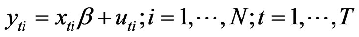 (1)
(1)
where the index i denotes N regional units and the index t refers to the T observations of each region i. The i subscript, therefore, denotes the cross-sectional dimension whereas t denotes time-series dimension. The total number of observations is NT.  is the observation on the
  region over the
  time period;
  is the
  observation on k explanatory variables and
  is the regression disturbance term. The error term
  follows a two-way random effects with both regional specific and temporal effects; that is,
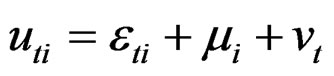 (2)
(2)
where  denotes regional specific effects,
  denotes temporal effects and
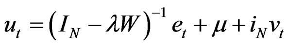
  represents the remainder disturbance term. Stacking the N observations of each timeperiod t, Equation (2) may be written as:
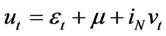 (3)
(3)
where ,
,  is a vector of ones of N dimension,
  and
and .
.
Assumption 1: Both  and
and  are assumed independent and normally distributed according to,
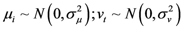 (4)
(4)
The remainder disturbance term  is assumed to follow the first order spatial error correlation (see [2,3]), that is:
 (5)
(5)
where  and
and . The term
  is the scalar spatial autoregressive coefficient with
 . The matrix W is an
  spatial weight matrix which represents the degree of potential interaction between neighboring locations whose diagonal elements are zero and off-diagonal elements are non-zero. Equation (5) can be further simplified as:
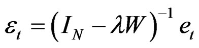 (6)
(6)
Given Equation (6), the weight matrix W also satisfies the condition that  is nonsingular for all
 .
.  is also assumed to be independent and normally distributed as:
 (7)
(7)
The  process is also independent of the
  and
and  terms.
The model (1) can be re-written in matrix notation as:
 (8)
(8)
where y is of dimension  vector, X is an
  matrix,
  is
is  vector and u is
  vector. The matrix X is assumed to be of full column rank and its elements are assumed to be asymptotically bounded in absolute value. Given Equation (6), Equation (3) can be re-written as:
 (9)
(9)
We can write Equation (8) in vector from as:
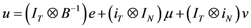 (10)
(10)
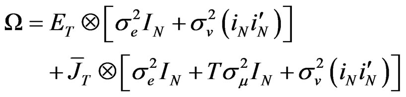
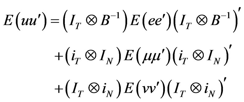
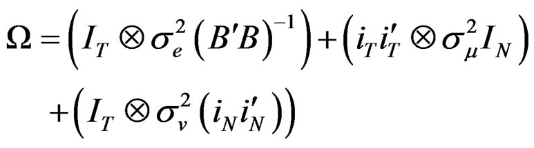
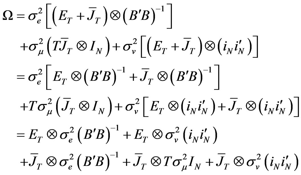
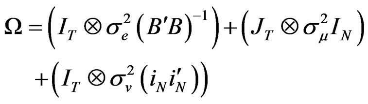
The variance-covariance (VCV) matrix  of Equation (10) (that is, the unrestricted model) can be expressed as:
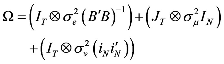 (11)2
(11)2
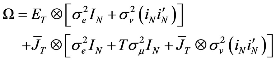
where  and it is a matrix of ones of dimension T. To obtain the spectral decomposition of Equation (11), we use the [24] method. Essentially, we replace
  by
by  and
and  by
by  where
where  and
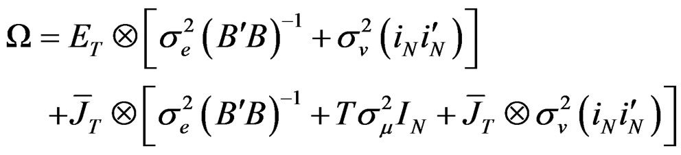
and  and consequently, we obtain3:
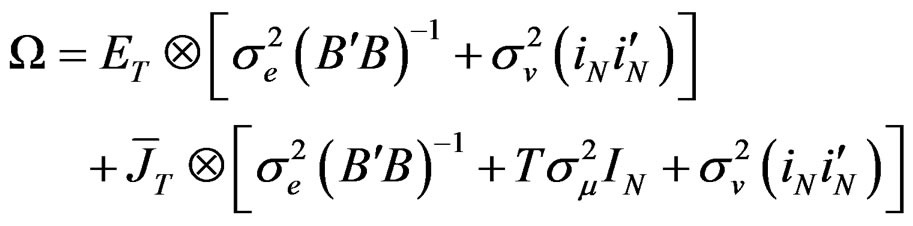 (12)
(12)
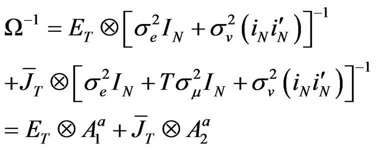
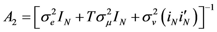
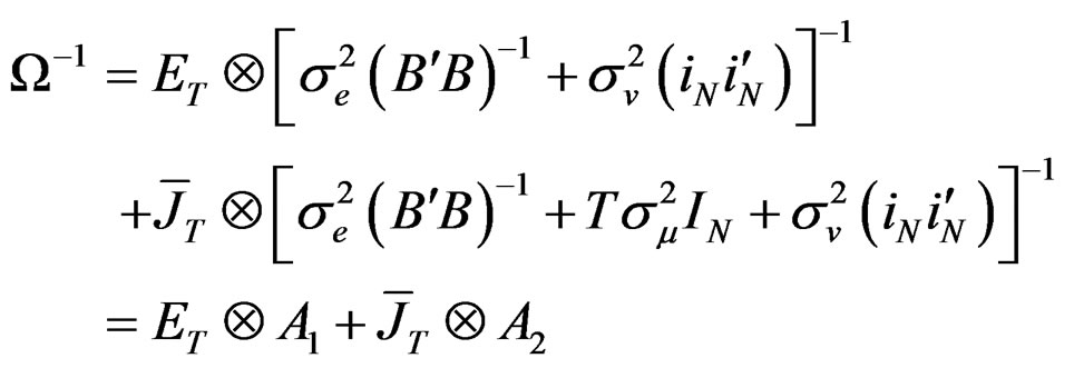
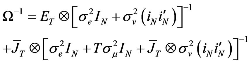
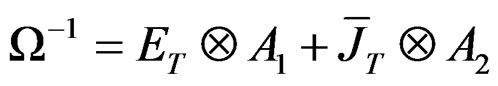
Also, using the [25] method of inversion, Equation (12) can be expressed as:
 (13)
(13)
where 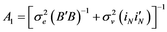 and
and
 .
.
3. Derivation of the LM Test
In this section, we derive the LM test for testing for no cross-sectional dependence in a two-way random effects model. We employ the Maximum Likelihood (ML) approach and consequently, the log-likelihood function. The LM test derived is based on the idea that the score of the likelihood function evaluated under the null is equal to zero when the null hypothesis is true, so that a  test based on the square of the score divided by the appropriate element of the information matrix (since this is the variance of the score) can be constructed. The use of the normal likelihood function requires the assumption of normality of the error term.
Essentially, the derivation of the LM test involves the following steps:
Step 1: Derive the VCV matrix for the unrestricted model;
Step 2: Derive the VCV matrix for the restricted model;
Step 3: Derive the spectral decomposition for the matrices obtained in steps 1 and 2;
Step 4: Derive the inverse of the matrices obtained in steps 1 and 2 using the results from step 3;
Step 5: Derive the general log-likelihood function;
Step 6: Use the information in steps 1 - 5 to derive the score functions of the likelihood evaluated from the restricted ML under ;
;
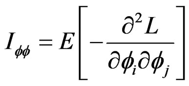
Step 7: Derive the information matrix and its inverse;
Step 8: Use the results obtained in steps 6 and 7 to develop the LM test.
The log likelihood function, L under normality of disturbances is given as:
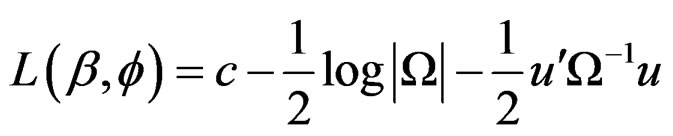 (14)
(14)
where 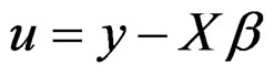 and the vector of parameters is denoted as
 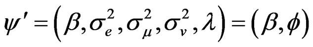 where
where
 .
.
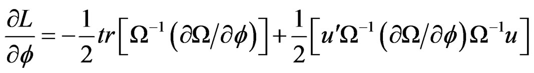
Since our test statistic requires information only on the vector of parameters , consequently, information due to
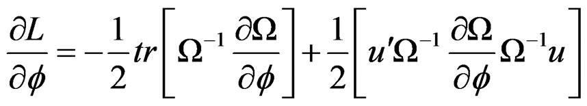
  is ignored. Following [26], the gradient of the log likelihood with respect to
  can be expressed as:
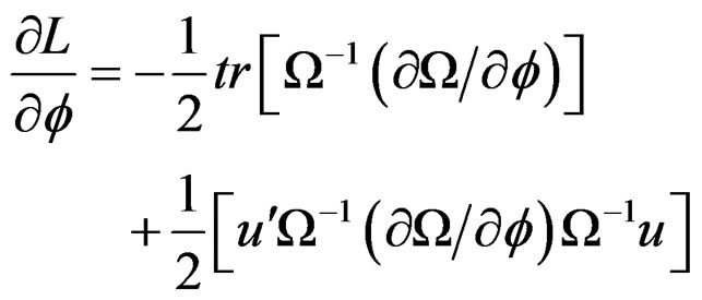 (15)
(15)
 (16)
(16)
By further simplification, it is easy to show that:
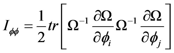
For  Equations (15) and (16) represent the score function and the information matrix respectively. The information matrix-
 is block diagonal. The LM statistic can, therefore, be written generally as:
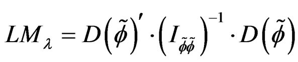
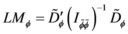 (17)
(17)
where  and
and  are the score function and information matrix respectively evaluated at the null hypothesis. The LM test statistic expressed in (17) is distributed as
  (i.e. chi-square distributed) with
  degrees of freedom,
  being the number of parameters in the vector
 . Based on Equation (17), therefore, the following hypotheses can be tested in relation to cross-sectional dependence:
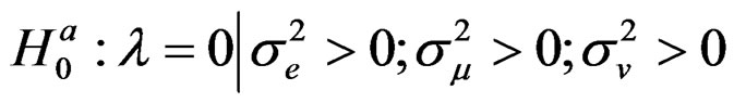 (18)
(18)
This is a test of no cross-sectional dependence assumeing the presence of random individual and time effects. This is the null hypothesis this study sets out to test.
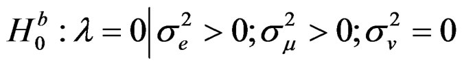 (19)
(19)
This hypothesis tests for cross-sectional dependence assuming the presence of random individual effect only (while ignoring the presence of time effects). This test is similar to [1] LM test for spatial error correlation as well as random country effects.
 (20)
(20)
This hypothesis tests for cross-sectional dependence ignoring the presence of both the random country and time effects. This is similar to the LM test by [2,4].
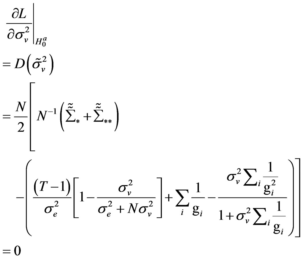
We derive below the score function for the null hypothesis expressed in (18) above which is the focus of this paper; that is:

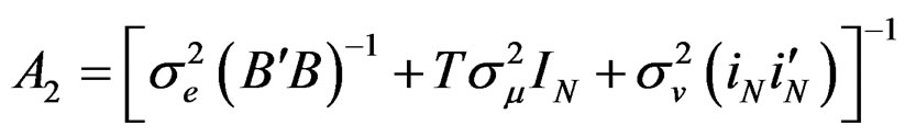
Under the null hypothesis in (18), the VCV matrix reduces to:4
 (21)
(21)
Given that ; then
  and, therefore,
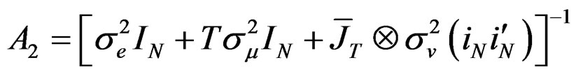
 . The Equation (21) is the VCV matrix for the restricted model. Using [25] Lemma 2.1, the inverse of Equation (21) can be expressed as:
 (22)
(22)
where 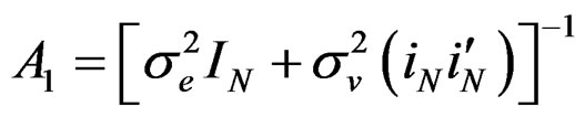 and
and
 .
.
The Equation (22) is the reduced form of Equation (13) and is also the VCV matrix for the familiar two-way random effects error components model. In addition, it is a principal component required in the log-likelihood function to derive the LM test. In particular, both Equations (21) and (22) are required to derive the partial derivatives and information matrix for the LM test.
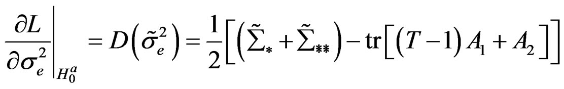
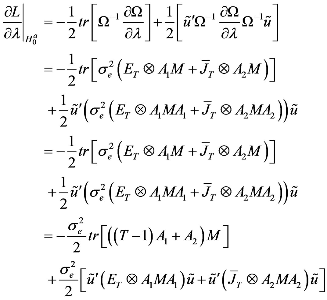
Using the general formulas on log likelihood differentiation, we derive its gradients evaluated at the restricted ML under  as follows:
Recall Equation (15):
Assumption 2: Let , then
 . Recall,
  and since under
 ,
, ; then
  and
and .
.
Assumption 3: If  are idempotent and symmetric matrices, we can write that
  where
where . Then,
  and
and  are orthogonal (see [3]).
Proposition 1: Based on assumptions 2 and 3, we can write the derivatives  for the parameters,
  ,
,
 ,
,  and
and , respectively, as:
Proof:
 (24)
(24)
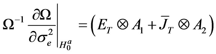
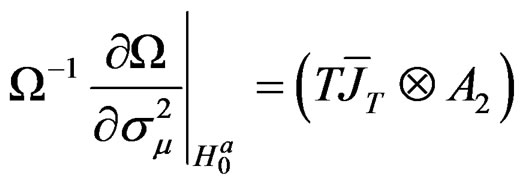
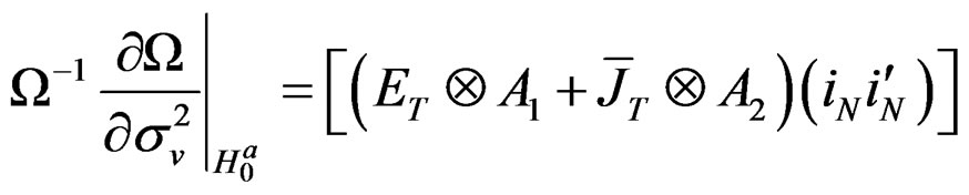
Based on assumption 1, it is easy to establish from Equation (24) that:
 (25)5
(25)5
 (26)
(26)
 (27)
(27)
 (28)
(28)
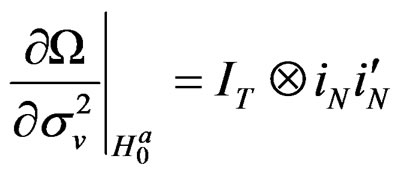
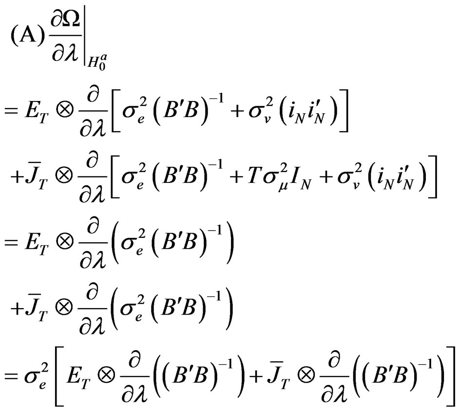
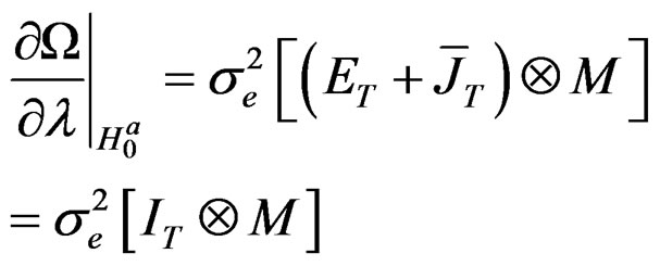
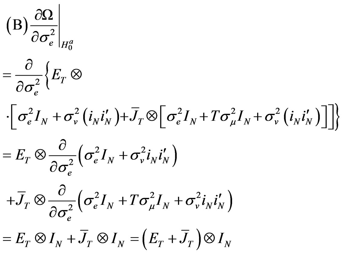
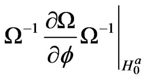
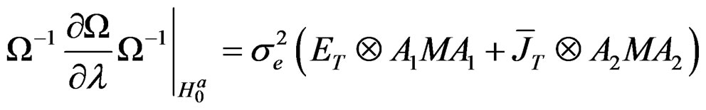
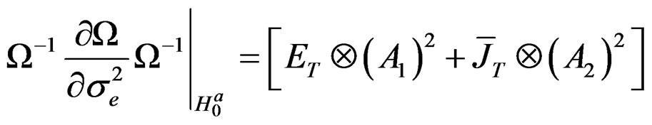
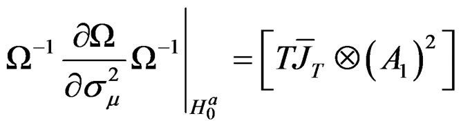
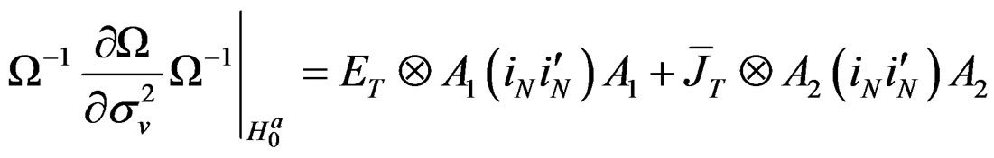
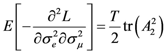
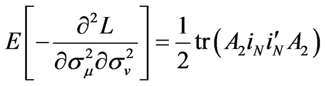
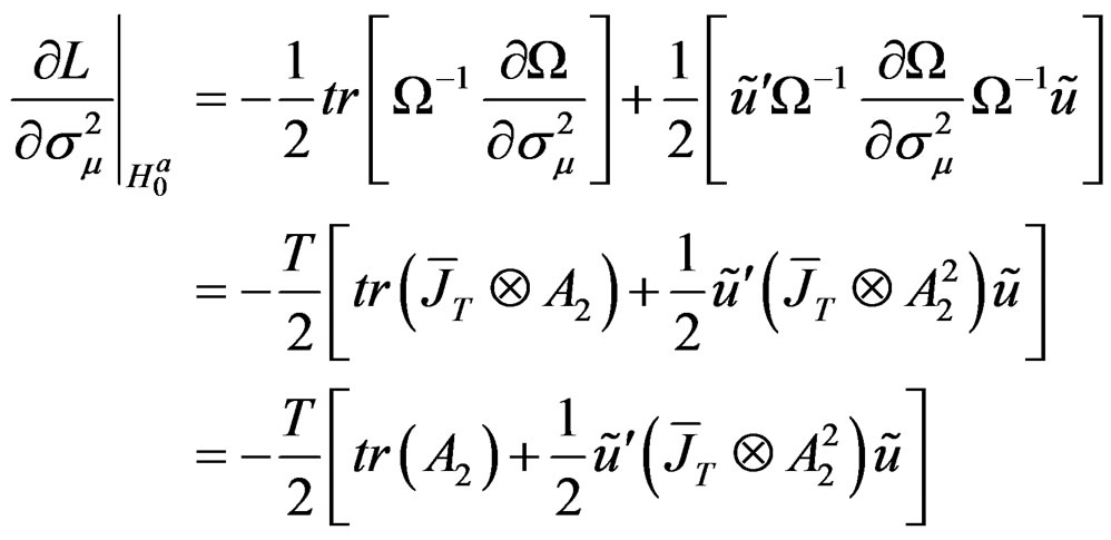
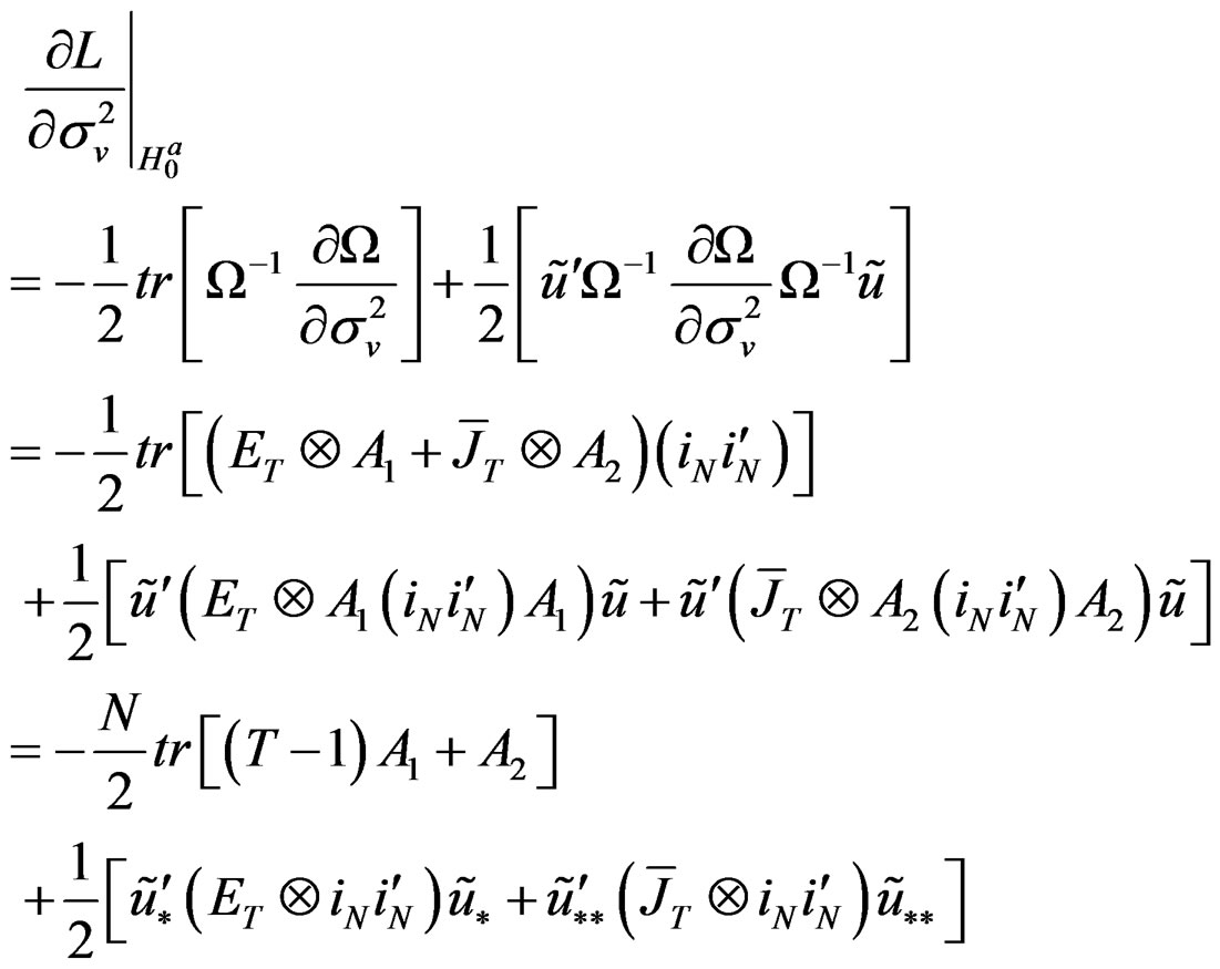
Proposition 2: Based on proposition 1 and assumptions 2 and 3, we can write the derivations of 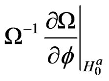 for the parameters,
  ,
,  ,
,  and
and , respectively, as:
wang#title3_4:spProof:
These derivatives are quite straightforward to show particularly using the information in proposition 1.
Proposition 3: Based on propositions 1 and 2 and assumptions 2 and 3, we can write the derivations of
 for the parameters,
  ,
,  ,
,  and
and
 , respectively, as:
wang#title3_4:spProof:
These derivatives are straightforward to show using the information in proposition 2.
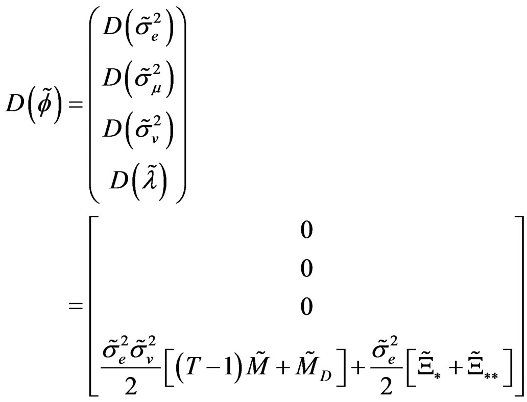
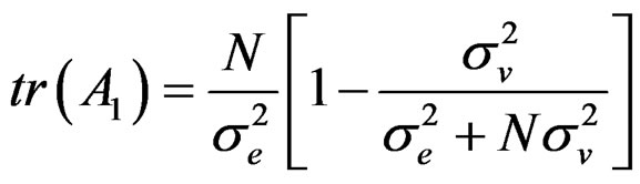
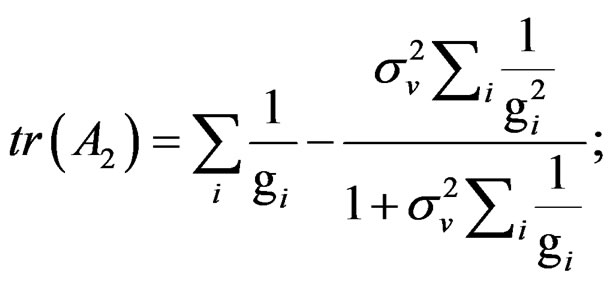
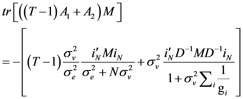
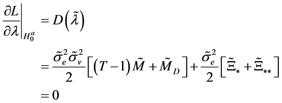
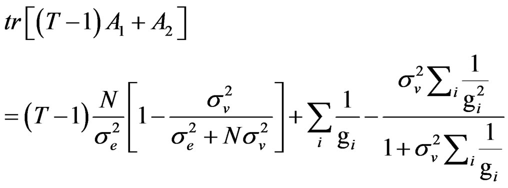
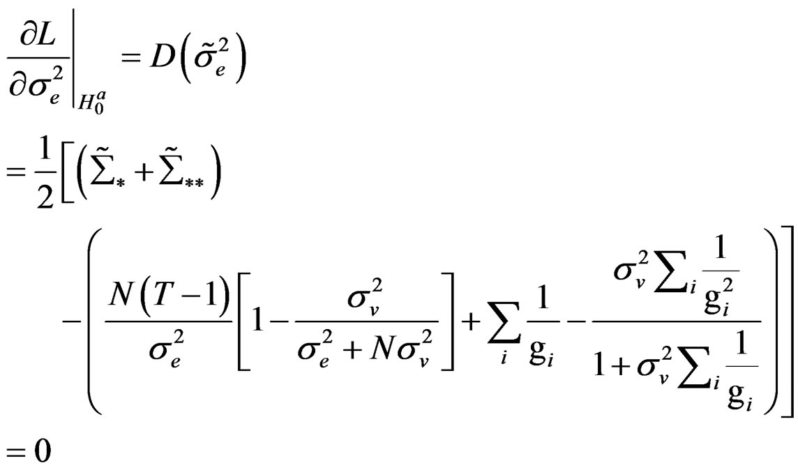
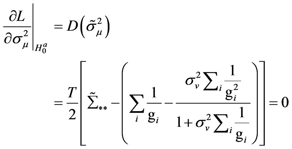
Proposition 4: Following propositions 1 - 3, we can easily calculate the partial derivates 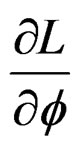 for
for
 ,
, 
and , respectively, evaluated at the restricted MLE:
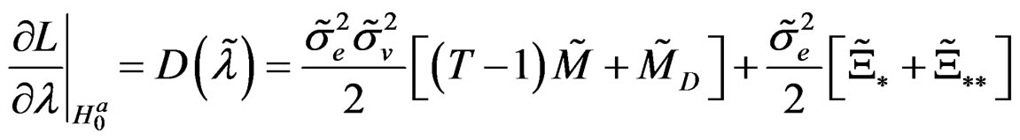
where ;
; 
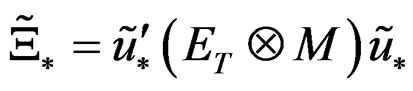 ;
;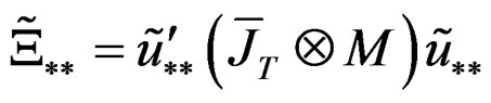
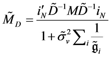
where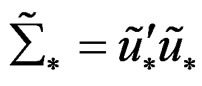 ;
;  and
and .
.
where  and
and
 .
.
Proof:
See the appendix for further simplifications and proofs of the partial derivatives.
Recall that we define , thereforeunder
 ,
,  can be defined as the solution obtained after maximization of the first order condition and
  is the corresponding residual under
 . Note that all the parameters
 were evaluated when
 at the restricted MLE except
  . This is because we are testing whether
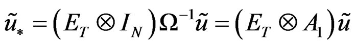
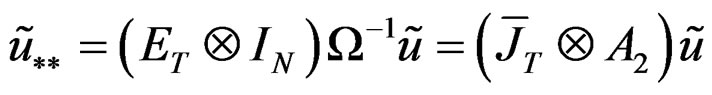
  is statistically different from zero. Thus, the partial derivatives under
  are rewritten in vector form as:
Also, using the method developed by [27], we obtain the information matrix under . The information matrix is given by:
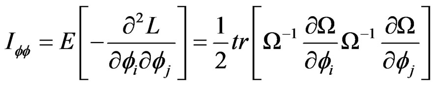 (29)
(29)
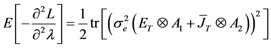
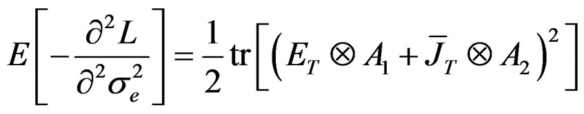
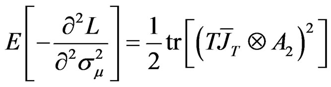
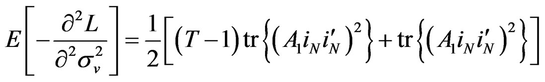
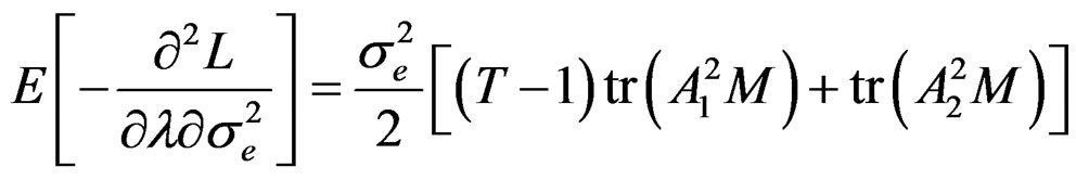
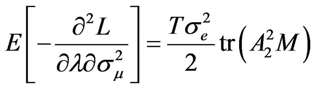
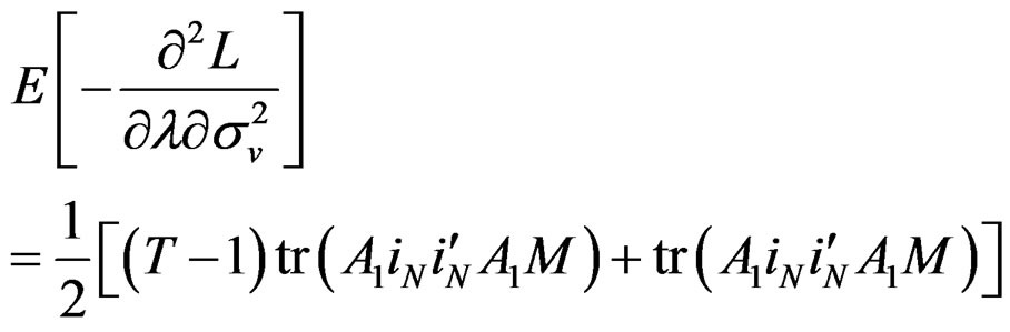
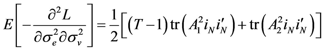
Proposition 5: Using the formular expressed in Equation (29) and information in proposition 2, we can derive respective elements in  under
under  for the vector of parameters
  as follows:
Given these information under , the LM statistic is given by,6
 (30)
(30)
Under  is distributed as
 . The statistic expressed in (30) is the LM test statistic, which tests for no cross-sectional dependence in a two-way random effects model.
Decision Criteria:
The LM statistic is a scalar and the value obtained when the test is performed on the two-way error components model is compared with the critical value for the chi-squared distribution— . The intention is to ascertain whether to reject the null hypothesis,
  , that there is no cross-sectional dependence problem in a two-way random effects model. Essentially, if
  is less than the critical value for the chi-squared distribution, then, we do not reject the null hypothesis implying that there is no cross-sectional dependence; otherwise, we reject it.
4. Concluding Remarks
This paper provides a framework for testing for no crosssectional dependence assuming the presence of random individual and time effects. Thus, several important issues have not been incorporated. These include testing other hypotheses earlier specified, that is;  which tests for crosssectional dependence assuming the presence of random individual effect only (while ignoring the presence of time effects; and
 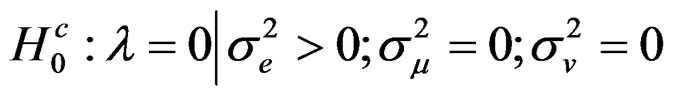 which tests for cross-sectional dependence ignoring the presence of both the random country and time effects. Also, the empirical applications section involving Monte Carlo experiments is also not yet considered. These are some of the suggestions for future research.
REFERENCES
- B. H. Baltagi, S. H. Song and W. Koh, “Testing Panel Data Regression Models with Spatial Error Correlation,” Journal of Econometrics, Vol. 117, No. 1, 2003, pp. 123- 150. doi:10.1016/S0304-4076(03)00120-9
- L. Anselin, “Rao’s Score Tests in Spatial Econometrics,” Journal of Statistical Planning and Inference, Vol. 97, No. 1, 2001, pp. 113-139. doi:10.1016/S0378-3758(00)00349-9
- B. H. Baltagi, “Econometric Analysis of Panel Data,” 6th Edition, Wiley, Chichester, 2008.
- L. Anselin, “Spatial Econometrics: Methods and Model,” Kluwer Academic Publishers, Dordrecht, 1988.
- L. Anselin and S. Rey, “Properties of Tests for Spatial Dependence in Linear Regression Models,” Geographical Analysis, Vol. 23, No. 2, 1991, pp. 112-131. doi:10.1111/j.1538-4632.1991.tb00228.x
- J. Ord, “Estimation Methods for Models of Spatial Interaction,” Journal of the American Statistical Association, Vol. 70, No. 349, 1975, pp. 120-126. doi:10.2307/2285387
- A. Brandsma and R. Ketellapper, “Further Evidence on Alternative Procedures for Testing of Spatial Autocorrelation among Regression Disturbances,” In: C. Bartels and R. Ketellapper, Eds., Exploratory and Explanatory Analysis in Spatial Data, Martinus Nijhoff, Boston, 1979, pp. 11-36. doi:10.1007/978-94-009-9233-7_5
- H. Bloommestein, “Specification and Estimation of Spatial Econometric Models: A Discussion of Alternative Strategies for Spatial Economic Modeling,” Regional Science and Urban Economics, Vol. 13, No. 2, 1985, pp. 251-270. doi:10.1016/0166-0462(83)90016-9
- H. Kelejian and I. R. Prucha, “A Generalized Moments Estimator for the Autoregressive Parameter in a Spatial Model,” International Economic Review, Vol. 40, No. 2, 1999, pp. 509-533. doi:10.1111/1468-2354.00027
- H. H. Kelejian, I. R. Prucha and E. Yusefovich, “Instrumental Variable Estimation of A Spatial Autoregressive Model with Autoregressive Disturbances: Large and Small Sample Results,” In: J. LeSage and R. K. Pace, Eds., Spatial and Spatiotemporal Econometrics (Advances in Econometrics), Vol. 18, Elsevier, New York, 2004, pp. 163-198. doi:10.1016/S0731-9053(04)18005-5
- R. Haining, “Spatial Data Analysis in the Social and Environmental Sciences,” Cambridge University Press, Cambridge, 1988.
- L. Anselin and A. K. Bera, “Spatial Dependence in Linear Regression Models with an Introduction to Spatial Econometrics,” In: A. Ullah and D. E. A. Giles, Eds., Handbook of Applied Economic Statistics, Marcel Dekker, New York, 1998.
- P. Burridge, “On the Cliff-Ord Test for Spatial Autocorrelation,” Journal of the Royal Statistical Society, Vol. 42, 1980, pp. 107-108.
- J. S. Huang, “The Autoregressive Moving Average Model for Spatial Analysis,” Australian Journal of Statistics, Vol. 26, No. 2, 1988, pp. 169-178. doi:10.1111/j.1467-842X.1984.tb01231.x
- A. Case, “Spatial Patterns in Household Demand,” Econometrica, Vol. 59, No. 4, 1991, pp. 953-965. doi:10.2307/2938168
- K. V. Mardia and R. J. Marshall, “Maximum Likelihood Estimation of Models for Residual Covariance in Spatial Regression,” Biomerika, Vol. 71, No. 1, 1984, pp. 135- 146. doi:10.1093/biomet/71.1.135
- K. V. Mardia, “Maximum Likelihood Estimation for Spatial Models,” In: D. A. Griffith, Ed., Spatial Statistics: Past, Present and Future, Institute of Mathematical Geography, Ann Arbor, 1990, pp. 203-251.
- H. Kelejian and D. P. Robinson, “Spatial Correlation: A Suggested Alternative to the Autoregressive Model,” In: L. Anselin and R. Florax, Eds., New Directions in Spatial Econometrics, Springer-Verlag, Berlin, 1995, pp. 75-95. doi:10.1007/978-3-642-79877-1_3
- L. Anselin and R. Moreno, “Properties of Tests for Spatial Error Components,” Regional Science and Urban Economics, Vol. 33, No. 5, 2003, pp. 595-618. doi:10.1016/S0166-0462(03)00008-5
- L. Anselin, “Some Robust Approaches to Testing and Estimation in Spatial Econometrics,” Regional Science and Urban Economics, Vol. 20, No. 2, 1990, pp. 1-17. doi:10.1016/0166-0462(90)90001-J
- H. Kelejian and I. R. Prucha, “A Generalized Spatial Two Stage Least Squares Procedure for Estimating a Spatial Autoregressive Model with Autoregressive Disturbances,” Journal of Real Estate Finance and Economics, Vol. 17, No. 1, 1998, pp. 99-121. doi:10.1023/A:1007707430416
- B. H. Baltagi, S. H. Song, B. C. Jung and W. Koh, “Testing for Serial Correlation, Spatial Autocorrelation and Random Effects Using Panel Data,” Journal of Econometrics, Vol. 140, No. 1, 2007, pp. 5-51. doi:10.1016/j.jeconom.2006.09.001
- B. H. Baltagi, S. H. Song and J. H. Kwon, “Testing for Heteroscedasticity and Spatial Correlation in a Random Effects Panel Data Model,” Computational Statistics and Data Analysis, Vol. 53, No. 8, 2009, pp. 2897-2922. doi:10.1016/j.csda.2008.06.009
- T. J. Wansbeek and A. Kapteyn, “A Simple Way to Obtain the Spectral Decomposition of Variance Components Models for Balanced Data,” Communications in Statistics, Vol. 11, No. 18, 1982, pp. 2105-2112. doi:10.1080/03610928208828373
- J. R. Magnus, “Multivariate Error Components Analysis of Linear and Nonlinear Regression Models by Maximum Likelihood,” Journal of Econometrics, Vol. 19, No. 2-3, 1982, pp. 239-285. doi:10.1016/0304-4076(82)90005-7
- J. R. Magnus and H. Neudecker, “Matrix Differential Calculus with Applications in Statistics and Econometrics,” Wiley Series in Probability and Statistics, Chichester, 1988.
- D. A. Harville, “Maximum Likelihood Approaches to Variance Component Estimation and to Related Problems,” Journal of the American Statistical Association, Vol. 72, No. 358, 1977, pp. 320-338. doi:10.2307/2286796
Appendix
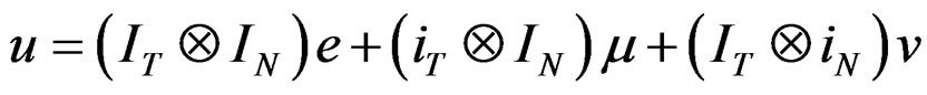
(A) Derivation of the VCV Matrix for the Unrestricted Model
Here,  and the VCV matrix of u can be derived as follows.
Recall Equation (10),

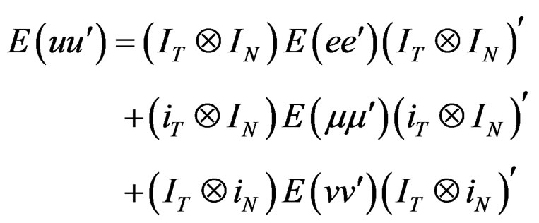
Using assumption (1), the VCV matrix can be expressed as:
 (A.1)
(A.1)
Let  in this case be represented by
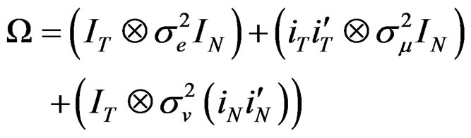
 , and by further simplification, (A.1) becomes:
 (A.2)
(A.2)
 (A.3)
(A.3)
where  and it is a matrix of ones of dimension T. To obtain the spectral decomposition of (A.3), we use the [24] method which involves replacing
  by
by  and
and  by
by  where
where  and
and  in (A.3). This is done as follows:
 (A.4)
(A.4)
Using the [25] method of inversion, therefore, the inverse of Equation (A.5) can be expressed as:
 (A.5)
(A.5)
where  and
and

(B) Derivation of the VCV Matrix for the Restricted Model
Here,  and as a consequence,
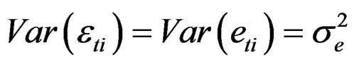 . Given this assumption, Equation (10) reduces to:
 (B.1)
(B.1)
Then, using assumption (1), the VCV matrix can be expressed as:
 (B.2)
(B.2)
Thus, (A.4) under the unrestricted model reduces to:
 (B.3)
(B.3)
 (B.4)
(B.4)
Just as before, we use the [24] method to obtain the spectral decomposition of (B.4) and following the same procedure as Appendix A, we have:
 (B.5)
(B.5)
Similarly, using the [25] method of inversion,  can be expressed as:
 (B.6)
(B.6)
where  and
and
 .
.
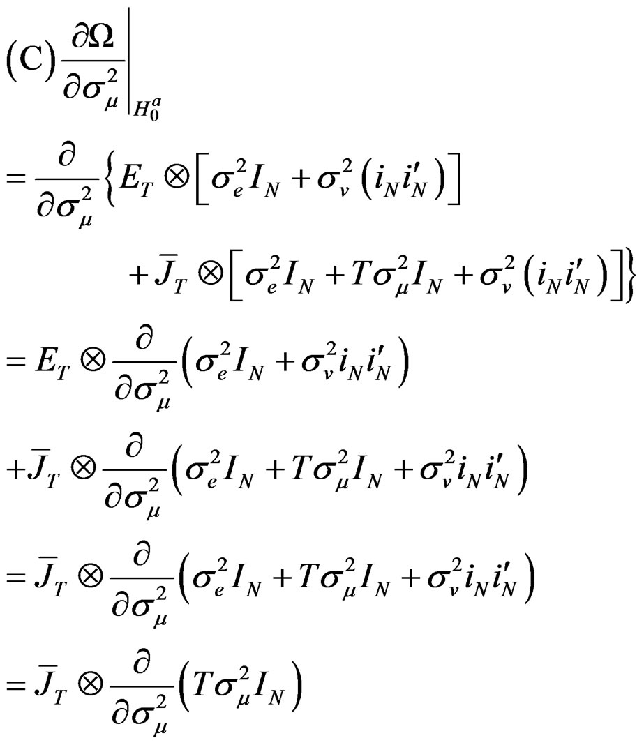
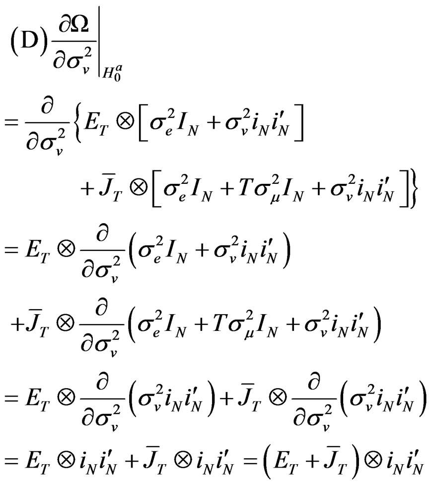
(C) Derivation of the Partial Derivatives 
(C.1)
Note that:
where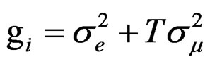 .
.
Therefore,

By some algebraic simplifications, we can write that:
Note further that:

in which case,
 therefore;
Similarly,
in which case,
 therefore;
 .
.
As a consequence, we can write (C.1) as:
 (C.2)
(C.2)
where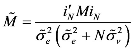 ;
; 
Using the information leading to (C.2), we can prove that:
And also with the representations that:
 in which case,
 therefore;
 ;
;
and in the same vein,
 .
.
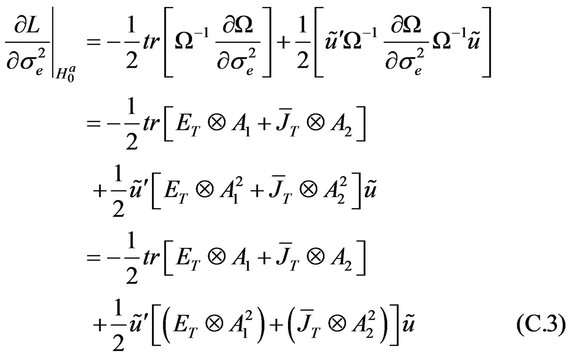
Given this information therefore, (C.3) becomes:
(C.4)
 (C.5)
(C.5)
Using the information that:
 ;
;
and

(C.5) becomes,
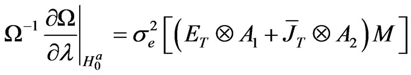
 (C.6)
(C.6)
(C.7)
where  and
and
 .
.
NOTES
1A review of score test statistics for alternative specifications in spatial econometrics in the context of cross sectional data and one-way error components model can be found in [2,3] respectively.
2See the appendix for the derivation.
3Note that  and
and  are symmetric idempotent matrices.
4See the appendix for the derivation.
5We also replace  by
by  where
where .
.
6Details of derivations of the information matrix can be provided on request.