Open Journal of Statistics
Vol.1 No.3(2011), Article ID:8072,7 pages DOI:10.4236/ojs.2011.13024
Bias of the Random Forest Out-of-Bag (OOB) Error for Certain Input Parameters
Metabolon Inc., Research Triangle Park, New Caledonia, USA
E-mail: mmitchell@metabolon.com
Received June 8, 2011; revised July 10, 2011; accepted July 18, 2011
Keywords: Random Forest, Multivariate Classification, Metabolomics, Small n Large p
Abstract
Random Forest is an excellent classification tool, especially in the omics sciences such as metabolomics, where the number of variables is much greater than the number of subjects, i.e., “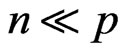 ”. However, the choices for the arguments for the random forest implementation are very important. Simulation studies are performed to compare the effect of the input parameters on the predictive ability of the random forest. The number of variables sampled, m-try, has the largest impact on the true prediction error. It is often claimed that the out-of-bag error (OOB) is an unbiased estimate of the true prediction error. However, for the case where
 , with the default arguments, the out-of-bag (OOB) error overestimates the true error, i.e., the random forest actually performs better than indicated by the OOB error. This bias is greatly reduced by subsampling without replacement and choosing the same number of observations from each group. However, even after these adjustments, there is a low amount of bias. The remaining bias occurs because when there are trees with equal predictive ability, the one that performs better on the in-bag samples will perform worse on the out-of-bag samples. Cross-validation can be performed to reduce the remaining bias.
1. Introduction
Random forest [1] is an ensemble method based on aggregating predictions from a large number of decision trees. Some of the advantages of random forest classification are the following: it is invariant to transformation, it is resistant to outliers, it does not overfit the data, it is fairly easy to implement with available software, and it works well when the number of subjects, n, is much fewer than the number of variables, p, i.e., “![]() .” Breiman discusses the properties of random forest for the various input parameters in his seminal paper [1]. However, in this discussion, the number of samples was larger than the number of variables. Thus, these properties may differ when
.” Breiman discusses the properties of random forest for the various input parameters in his seminal paper [1]. However, in this discussion, the number of samples was larger than the number of variables. Thus, these properties may differ when![]() . Strobl et al. [2] have observed that there is bias in variable selection when subsampling with replacement (the default) is used, but the effect on the out-of-bag (OOB) error is not assessed. It is often stated that the OOB error is an unbiased estimate of the true prediction error. However, we will show that this is not necessarily the case.
. Strobl et al. [2] have observed that there is bias in variable selection when subsampling with replacement (the default) is used, but the effect on the out-of-bag (OOB) error is not assessed. It is often stated that the OOB error is an unbiased estimate of the true prediction error. However, we will show that this is not necessarily the case.
In this manuscript, we compare the effect on the prediction error for different choices of the input parameters: 1) for subsampling with versus without replacement (the replace parameter); 2) the proportions of observations used for the in-bag samples (the sampsize parameter); and 3) various values of the number of variables sampled (the m-try parameter). These are compared for various simulated data sets with varying dimensions. Additionally, for each of these scenarios we compare the OOB error to the true prediction error where the choice of these parameters can cause a severe overestimation of the true error. This is in contrast to many methods, which can easily overfit the data and underestimate the true prediction error.
2. Simulation Study
To compare the effects of various input parameters on the OOB error estimate and the true prediction error, various models are simulated. Three models are compared: 1) a model of random noise; 2) a model with 20 true predictors; and 3) a model with 40 true predictors and correlated variables. More specific details for each model are given below. All models are simulated for p = 400 variables, and for two groups with sizes n1 = n2 = 6, n1 = n2 = 10, and n1 = n2 = 30. The dimensions of the data sets were chosen to mimic metabolomics data: rat studies typically have 10 or fewer rats per group, and groups of size 30 are more common for human studies. Subsampling with replacement (the default) and subsampling without replacement are compared for various proportions of in-bag observations (the default is approximately 63% of the total observations). The m-try parameter was set to 4, 20 (the default, which is the square root of the number of variables), 200 and 400 (all variables).
The value of m-try made no difference for the conclusions for the random noise model, Model 1, so the results are shown only for m-try = 20, the default. For each random forest, 1000 trees were used. For each combination, 500 simulation runs were performed. For each simulated data set, a test set with the same dimensions was simulated, so that the OOB estimate of the error can be compared to the actual prediction error. All simulations were performed with R [3], using the randomForest package [4].
The results for Model 1 for n1 = n2 = 6, n1 = n2 = 10, and n1 = n2 = 30 are shown in Tables 1-3, while the results for Models 2 and 3 are shown in Tables 4-6, and Tables 7-9, respectively. Each entry in the table represents the average value across the simulation runs, and in parentheses, the margin of error for a 95% confidence interval is given (i.e., ). The bias is the average OOB error minus the average test set prediction error. The “N” column represents the sampsize argument.
Simulated Models
Model 1
This model is random noise: there are 400 independent normal random variables with mean zero and standard deviation equal to 0.3 for each group.
Model 2
This model has 20 true predictors with independent errors. More formally for Group 1, X = (X1, ..., X400)' is multivariate normal with mean vector (0.26 × 110, 0390) where 1p is a vector of p ones and 0q is a vector of q ze-
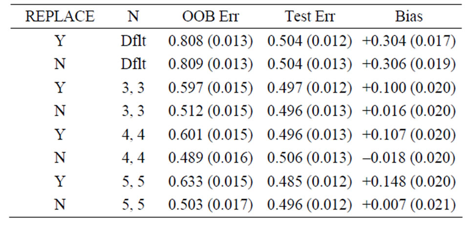
Table 1. Mean error rates for Model 1: random noise, n1 = n2 = 6, mtry = 20.
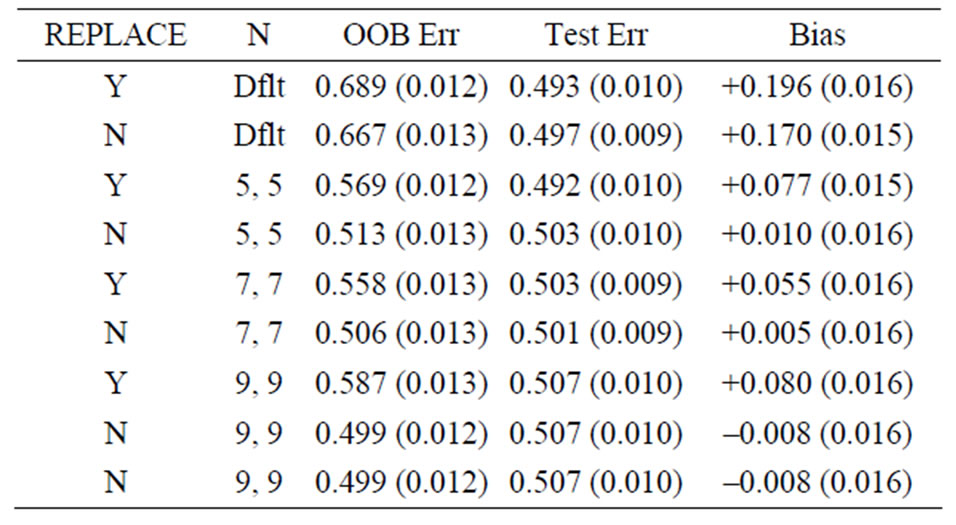
Table 2. Mean error rates for Model 1: random noise, n1 = n2 = 10, mtry = 20.
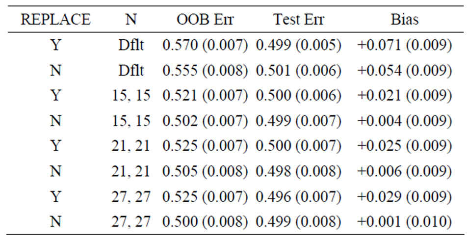
Table 3. Mean error rates for Model 1: random noise, n1 = n2 = 30, mtry = 20.
roes. The covariance matrix is (0.3)2 × I400 where I400 is the 400 by 400 identity matrix. Group 2 is identical except that the mean vector is (010, 0.26 × 110, 0380).
Model 3
This model has 40 true predictors with two clusters of five correlated variables each and two clusters of five correlated noise variables. More formally, for Group 1, X = (X1, ..., X400)' is multivariate normal with mean vector (0.26 × 120, 0380), and for Group 2, the mean vector is (020, 0.26 × 120, 0360). For each group, the covariance matrix is (0.3)2 × R with elements rij, where rii = 1. For i, j = 1, 2, ..., 5, rij = 0.9 for i ≠ j. For i, j = 21, 22, ..., 25, rij = 0.9 for i ≠ j. For i, j = 41, 42, ..., 45, rij = 0.9 for i ≠ j. For i, j = 51, 52, ..., 55, rij = 0.9 for i ≠ j. Otherwise, rij = 0.
3. Discussion
From all the tables, we see that the actual prediction error is similar for most of the combinations for each model, and the prediction error decreases with increasing sample sizes for Models 2 and 3. The sampsize parameter has little effect, but shows some degradation when 90% of the samples are used for the in-bag samples. The parameter with the largest impact on the true prediction accuracy is m-try, with the performance degrading for
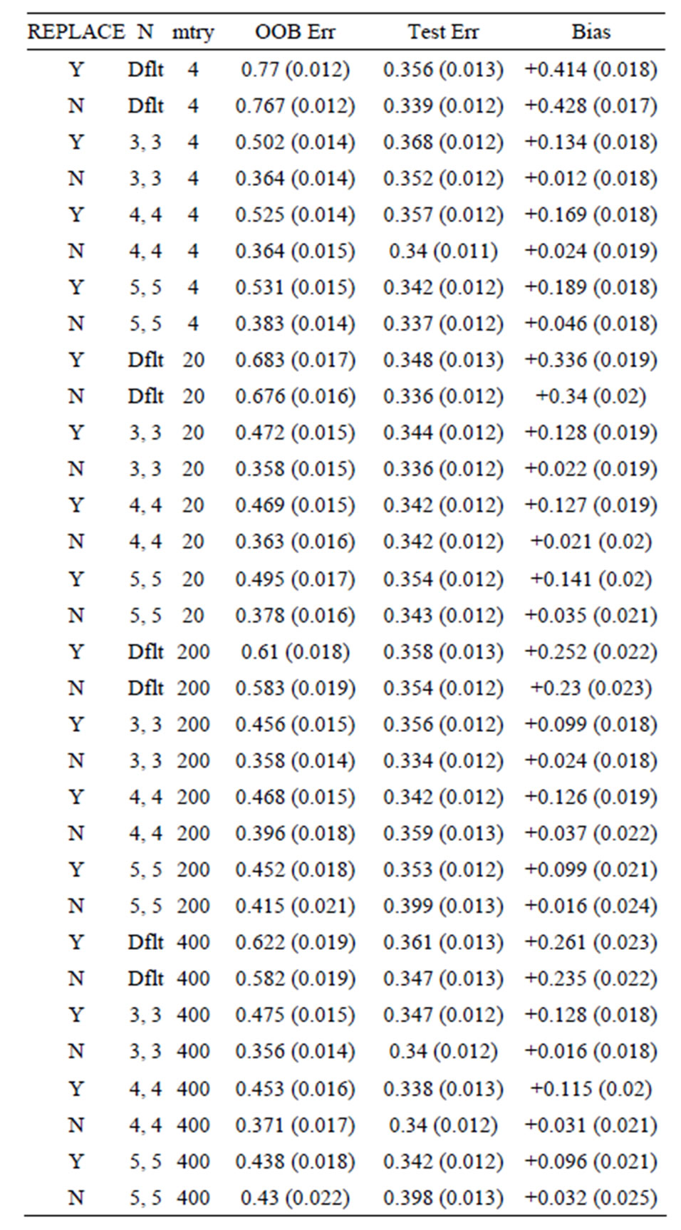
Table 4. Mean error rates for Model 2: 20 true predictors, n1 = n2 = 6.
the very large or very small values. However, the optimal choice of m-try will depend on the number of true predictors and their relationships.
For Model 1, the random noise model, the expected prediction error should be 50%. The true prediction errors, as measured by the average test set prediction errors, are indeed very close to 50%; however, the OOB error rates always overestimate the true error. With the default values of the inputs for the random forest function, the average OOB error is approximately 81% for n1 = n2 = 6 (see the first row of Table 1)! For the groups of sizes n1 = n2 = 10 and n1 = n2 = 30 the average OOB errors are 69% and 57%, respectively. This positive bias (i.e., the
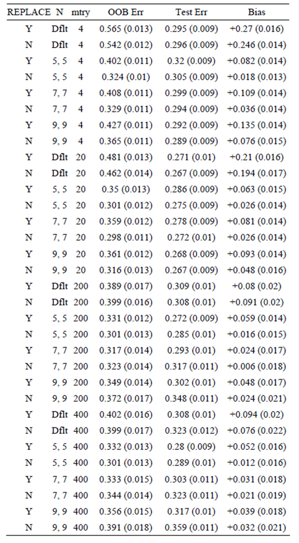
Table 5. Mean error rates for Model 2: 20 true predictors, n1 = n2 = 10.
OOB error is too pessimistic) is also seen for Models 2 and 3: for Model 2 the approximate biases are 34%, 21%, and 5%, for the groups of sizes n1 = n2 = 6, n1 = n2 = 10, and n1 = n2 =30, respectively; while for Model 3, the positive biases are approximately equal to 32%, 15%, and 3%, when n1 = n2 = 6, n1 = n2 = 10, and n1 = n2 =30, respectively. These results mirror those seen for the data sets with the group labels shuffled in [5], where the predictive ability of the variations of random forest are compared by using the OOB error rates for each. The OOB errors for the scrambled cases are much worse than random chance in most cases, with some OOB error rates equal to 75% and 83%. The data sets (gene arrays) used
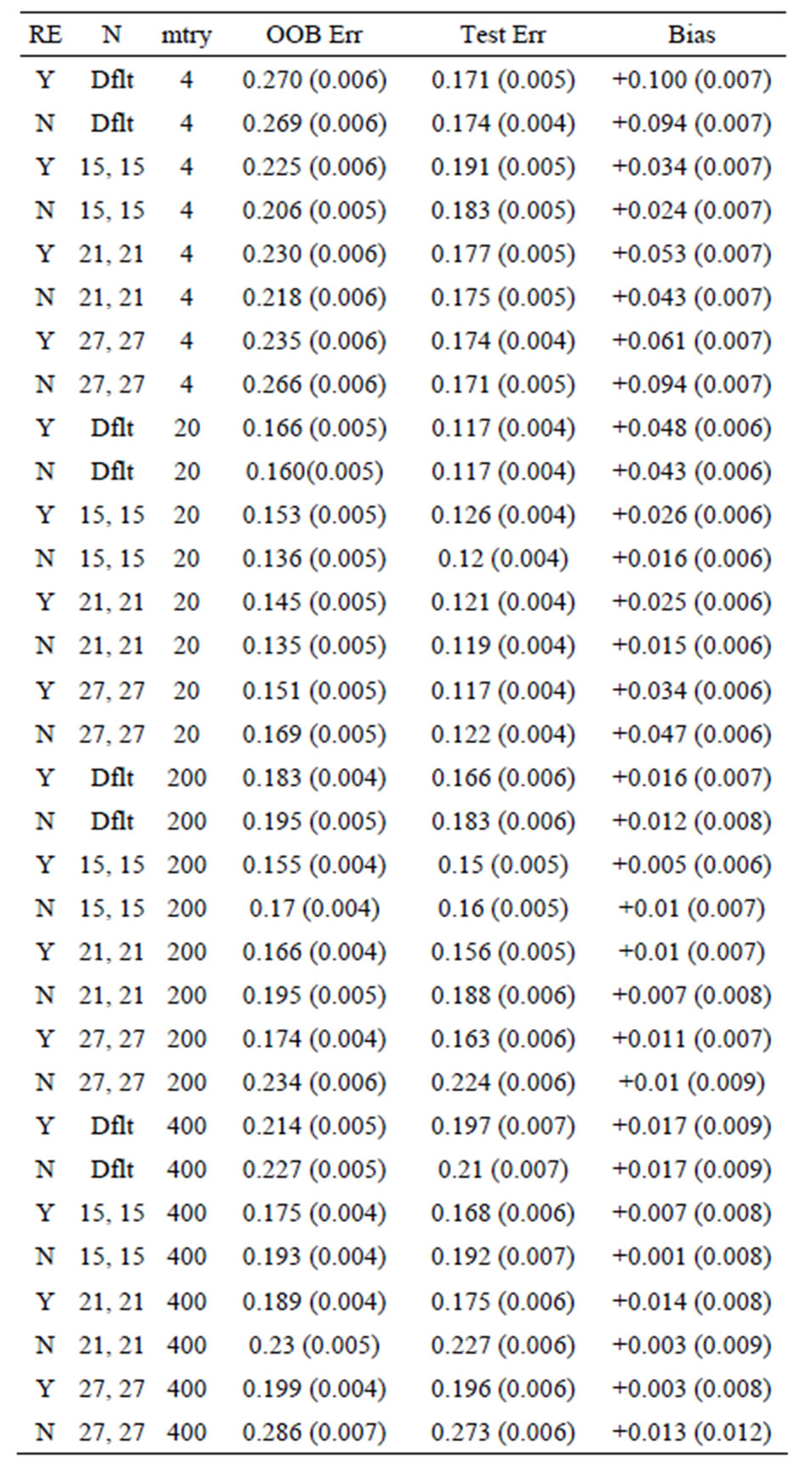
Table 6. Mean error rates for Model 2: 20 true predictors, n1 = n2 = 30.
in the paper have tens of thousands of variables with a very low number of subjects (10 - 35 total). In that paper, the default bootstrap sampling (sampling with replacement and not necessarily the same number chosen from each group) was used. Hence comparing the OOB error rates was not appropriate as these can be severely biased.
For a given sampsize argument, subsampling without replacement generally has a lower bias than subsampling with replacement (the default). Furthermore, when subsampling without replacement, forcing the same proportion to be sampled from each group reduces the bias over the default (no restriction of proportion for each group, only the total). This bias occurs because this subsampling
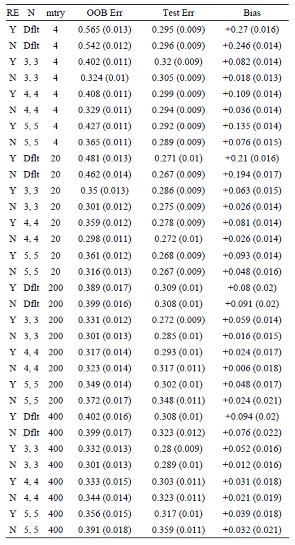
Table 7. Mean error rates for Model 3: 40 true predictors with correlations, n1 = n2 = 6.
will oversample from one of the two groups, so that an individual tree is weighted towards predicting that group over the other. However, the other group is more represented in the out-of-bag samples, resulting in predictions that appear worse than random chance. For example, suppose for two groups when n1 = n2 = 6 that the in-bag samples have five observations from Group 1 and one observation from Group 2. This tree will tend to predict most observations as belonging to Group 1, but the out-of-bag samples have one from Group 1 and five from Group 2. Such trees are created whenever the proportion of samples from each group is different for the in-bag samples, which results from subsampling with replace-
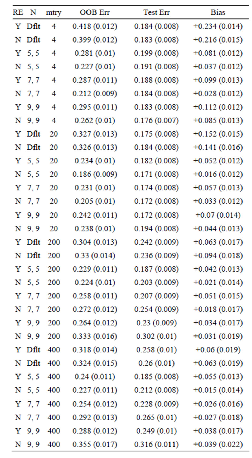
Table 8. Mean error rates for Model 3: 40 true predictors with correlations, n1 = n2 = 10.
ment or subsampling without replacement but not forcing the proportion sampled from each group to be the same.
From Tables 1-9 we see that the lowest biases occur when subsampling is performed without replacement and the proportion sampled from each group for the in-bag samples is the same. However, there is still bias remaining: the overwhelming majority of bias estimates are positive (each row represents an independent simulation run). The reason for this bias is more subtle: when there are variables of equal predictive ability on the whole data set, the one that performs worse on the out-of-bag samples for some combinations of in-bag observations will be chosen. To illustrate, two variables of equal predictive
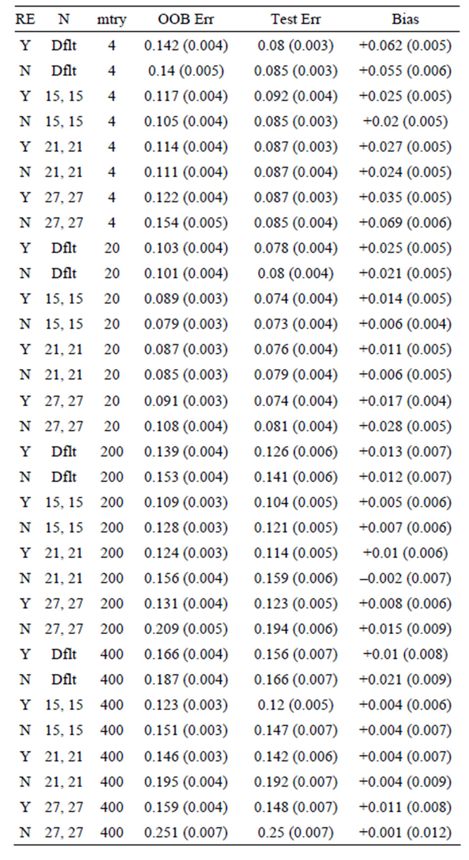
Table 9. Mean error rates for Model 3: 40 true predictors with correlations, n1 = n2 = 30.
ability for two groups of size five are shown in Table 10. We see that the decision trees X1 > 1 or X2 > 1 have equal predictive ability (20% error). Now, suppose the sampsize argument is set to (4, 4). For many combinations of in-bag samples, the performance of these trees is identical (e.g., in-bag samples 02 - 09). However, when samples 01 - 04 and 06 - 09 are chosen, X1 will be chosen over X2. This tree will be 100% accurate on the inbag samples. However, samples 05 and 10 will be predicted incorrectly. Likewise, if samples 02 - 05 and 07 - 10 are chosen, the scenario for X2 is identical. (Note: because, of the m-try argument, these two variables will not necessarily always be compared.) It can never be the case

Table 10. Two sample variables with equal predictive ability.
that with two variables of equal predictive ability that the one that performs worse on the in-bag samples but better on the out-of-bag samples will be chosen.
The modification of the random forest proposed by Strobl et al. [2] was also compared to see if the same behavior is exhibited. This implementation uses subsampling without replacement by default, so this source of bias is eliminated. Simulations were performed with the cforest function from the party library [2,6,7]. Since mtry = 20 performed well, this value was the only one used for these simulation runs. For sample sizes of six and ten per group, cforest failed to choose any variables and fit only the mean (resulting in 50% prediction accuracy on the test sets for every run for all three models). The results for the three models for the group size of 30 each are shown in Table 11, and we see a similar pattern to the bias as seen with the standard random forest. This is not surprising as the issue discussed in the previous paragraph applies here for the same reason.
To address the issue of the remaining bias, one can simply report the OOB error estimate an expected upper bound to the true prediction error, as the bias is fairly low when sampling without replacement and the same proportion from each group are chosen. Otherwise, cross-validation can be performed to further refine the error estimate. For Model 2, with n1 = n2 =30, mtry = 20, and 15 from each group was sampled without replacement, we also estimate the true prediction error using the average error obtained using leave-one-out cross-validation (LOO-CV). The results are shown in Table 12, and we see that the bias is zero as desired using LOO-CV
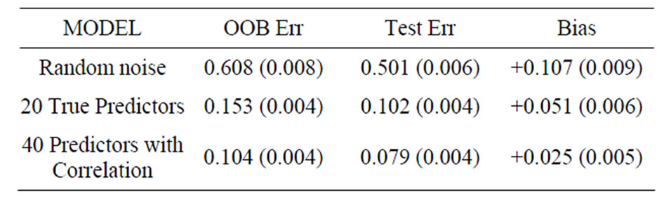
Table 11. Cforest results, mtry = 20, n1 = n2 = 30.

Table 12. Leave-one-out Cross-Validation Results for Model 2, n1 = n2 = 30, mtry = 20, subsampling 15 from each group without replacement.
(although the bias is low initially, so may make very little practical difference).
Finally we compare the OOB error for several of the genomics data sets shown in [5]. These data sets are available at http://www.rci.rutgers.edu/~cabrera/DNAMR, and consist of the “Astrocytoma” [8], “BreastCancer” [9], “Epilepsy” [10], and “HIV” [11] data sets. For each data set, subsampling without replacement was performed with sampsize set to 50% of the smaller group size (i.e., if the group sizes are 6 and 8, sampsize was set to (3,3), the default value of m-try was used, and 10,000 trees were used for each random forest. Each of these data sets has more than 10,000 variables. We compare the OOB error rates reported in [5], which were based on the default bootstrap sampling to those obtained using the recommended arguments (which are actually upper bounds as described above). In each case, the error rate was reduced over those given in [5]—many by 50%. The results are shown in Table 13.
4. Conclusions
Various models were simulated for a variety of combinations of input parameters (replace, sampsize, and m-try) and sample sizes for random forest in order to assess the performance of the out-of-bag (OOB) error estimate and the actual prediction error. The m-try parameter had the largest effect on the actual predictive ability, while the other parameters had little effect on the actual predictive ability in most cases. However, these parameters have a large effect on the OOB error estimate, which for certain parameters causes a severe positive bias. This bias is greatly reduced by subsampling without replacement and choosing the same proportion of observations from each group for the in-bag samples. There is still a small remaining positive bias that results from the variable selec-

Table 13. Comparison of OOB Error for genomics data sets given in [5] to those obtained using subsampling without replacement and sampling the name number from each group.
tion, and performing cross-validation can further refine the error estimate. However, since the bias is low, one may simply prefer to report the OOB error as an expected upper bound to the actual error.
5. References
[1] L. Breiman, “Random Forests,” Machine Learning, Vol. 45, No. 1, 2001, pp. 5-32. doi:10.1023/A:1010933404324
[2] C. Strobl, A. L. Boulesteix, A. Zeileis and T. Hothorn, “Bias in Random Forest Variable Importance Measures: Illustrations, Sources, and Solution,” BMC Bioinformatics, Vol. 8, Article 25, 2007. doi:10.1186/1471-2105-8-25 http://www.biomedcentral.com/1471-2105/ 8/25
[3] R Development Core Team, “R: A Language and Environment for Statistical Computing,” R Foundation for Statistical Computing, Vienna, 2008. http://www.R-project.org
[4] A. Liaw and M. L. Weiner, “Classification and Regression Trees by RandomForest,” R News 2002, Vol. 2, No. 3, 2002, pp. 18-22. http://www.webchem.science.ru.nl/PRiNS/ rF.pdf
[5] D. Amaratunga, J. Cabrera and Y.-S. Lee, “Enriched Random Rorests,” Bioinformatics, Vol. 24, No. 18, 2008, pp. 2010-2014. doi:10.1093/bioinformatics/btn356
[6] T. Hothorn, P. Buehlmann, S. Dudoit, A. Molinaro and M. Van Der Laan, “Survival Ensembles,” Biostatistics, Vol. 7, No. 3, 2006, pp. 355-373. doi:10.1093/biostatistics/kxj011
[7] C. Strobl, A. L. Boulesteix, T. Kneib, T. Augustin and A. Zeileis, “Conditional Variable Importance for Random Forests,” BMC Bioinformatics, Vol. 9, Article 307, 2008. doi:10.1186/1471-2105-9-307 http://www.biomedcentral.com/1471-2105/9/307
[8] T. MacDonald, “Human Glioblastoma,” 2001. http://pepr.cnmcrsearch.org/browse.do?action=list_prj_exp&projected=65
[9] M. Chan, X. Lu, F. Merchant, J. D. Iglehart and P. Miron, “Gene Expression Profiling of NMU-Induced Rat Mammary Tumors: Cross Species Comparison with Human Breast Cancer,” Carcinogenesis, Vol. 26, No. 8, 2005, pp. 1343-1353. doi:10.1093/carcin/bgi100
[10] D. N. Wilson, H. Chung, R. C. Elliott, E. Bremer, D. George and S. Koh, “Microarray Analysis of Postictal Transcriptional Regulation of Neuropeptides,” Journal of Molecular Neuroscience, Vol. 25, No. 3, 2005, pp. 285-298. doi:10.1385/JMN:25:3:285
[11] E. Masliah, E. S. Roberts, D. Langford, I. Everall, L. Crews, A. Adame, E. Rockenstein and H. S. Fox, “Patterns of Gene Dysregulation in the Frontal Cortex of Patients with HIV Encephalitis,” Journal of Neuroimmunology, Vol. 157, No. 1-2, 2004, pp. 163-175. doi:10.1016/j.jneuroim.2004.08.026