American Journal of Operations Research
Vol. 2 No. 4 (2012) , Article ID: 25151 , 9 pages DOI:10.4236/ajor.2012.24062
Optimal Stopping Time for Holding an Asset
Military Technical Academy, Hanoi, Vietnam
Email: van_khanh1178@yahoo.com
Received September 21, 2012; revised October 22, 2012; accepted November 3, 2012
Keywords: Optimal Stopping Time; Boundary; Brownian Motion; Black-Schole Model
ABSTRACT
In this paper, we consider the problem to determine the optimal time to sell an asset that its price conforms to the Black-Schole model but its drift is a discrete random variable taking one of two given values and this probability distribution behavior changes chronologically. The result of finding the optimal strategy to sell the asset is the first time asset price falling into deterministic time-dependent boundary. Moreover, the boundary is represented by an increasing and continuous monotone function satisfying a nonlinear integral equation. We also conduct to find the empirical optimization boundary and simulate the asset price process.
1. Introduction
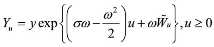
In [1], Shiryaev and Peskir have considered the problem:
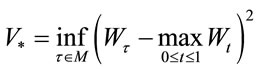 (1.1)
(1.1)
where  is standard Brownian process and they found the optimal stopping time as:
 (1.2)
(1.2)
where  is the solution of the equation

and .
.
The simulation for , boundary
  and
and  are given in Figures 1-3.
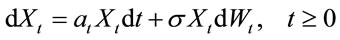
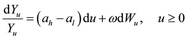
In [2], Albert Shiryaev, Zouquan Xu and Xun Yu Zhou solve the following problem: There is an investor holding a stock, and he needs to decide when to sell it for the last time with given time to sell T. It is obvious that he wants to sell at a time of highest price on the interval from 0 to T. Assume that the discounted share price  complies with the following dynamic equation:

on a filtered probability space  where a is the growth rate of the price and
  is the volatility, r is interest rate,
  is the standard Brownian motion with
  under the measure P. Here,
  is Pincreasing filter generated by
 . Then,
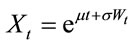
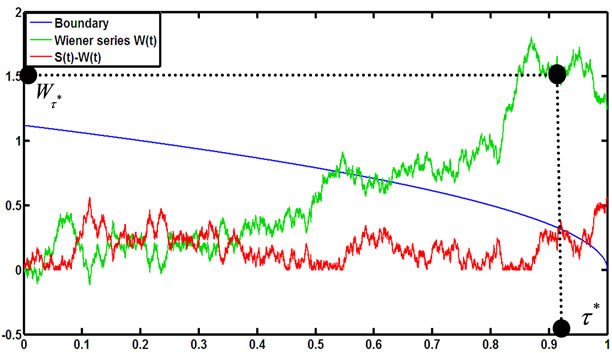
Figure 1. A simulation for stopping time in (1.2). The optimal stopping time  is the first time the boundary line (blue line) lies below the line describes the process
  (red line). In this case
  is very large but is not
 .
.

Figure 2. A simulation for the stopping time in (1.2). In this case  is less than 0 but is not
 .
.
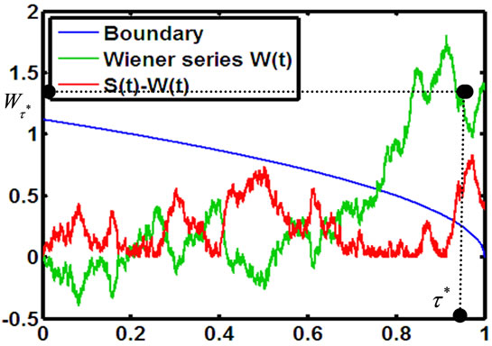
Figure 3. A simulation for the stopping time in (1.2). In this case  is very large but is not
 .
.
where
 . We define:
and .
.
Then, the following cases:
• If ,
,  is an unique optimal selling time.
• If ,
, or
or  are optimal selling times.
• If ,
,  is an unique optimal selling time.
In this paper, we will find the optimal time to sell a stock when the appreciation rate is the random variable taking one of two given values  and
and .
.
2. The Problem of Finding the Optimal Selling Time
Assume that the asset price process Xt follows a geometric Brownian motion with its drift is a random variable taking one of two given values  or
or , the volatility
  is constant, i.e.
 (2.1)
(2.1)
where  is a standard Brownian motion independent with
  of the probability space
 . Assume
  is a complete probability space with nondecrease
  -field. Suppose
  and
and  satisfy al < r < ah, where r is the interest rate and it is constant and the initial value of assets
  is a positive constant.
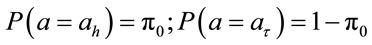
Investors holding assets need to decide when to sell it for the last time with given time to sell them is T. Knowing that at the initial time distribution of α as
At time  we put
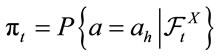 , where
  is the completion of the filtration generated by X.
The problem is finding  -stopping time τ, 0 ≤ τ ≤ T such that
 (2.2)
(2.2)
where supremum is taken in  -stopping time τ, 0 ≤ τ ≤ T.
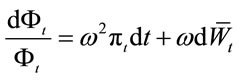
The price process  and posterior probability process
  satisfying the equations
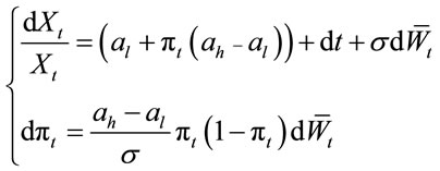 (2.3)
(2.3)
where  is a P-Brownian motion defined by:
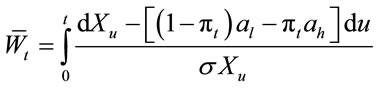
(see [3], theorem 9.1)
Define the process  by:
by:

and a new measure  satisfying:
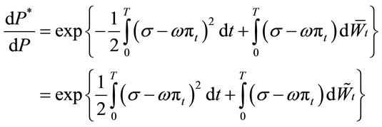
where .
.
According to the Girsanov theorem,  is a
is a  Brownian motion. Let
 , we have
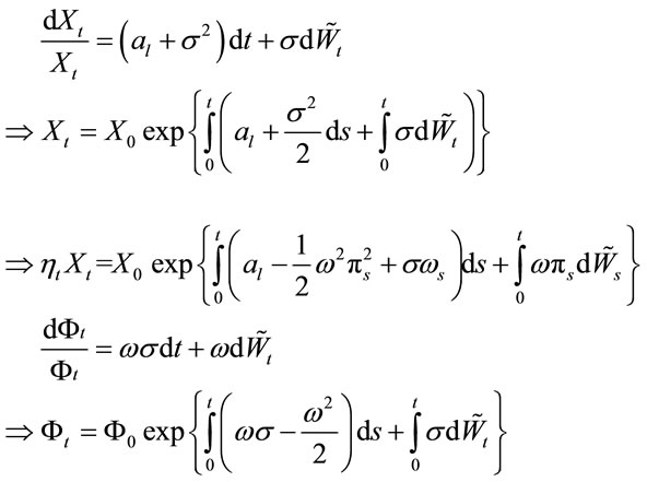
Then, price process  and process
  satisfy the equations
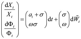 (2.4)
(2.4)
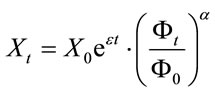
So, X and  are geometric Brownian motions under measure
 . Moreover,
  -field generated by
  coincides with the one generated by X.
We define the likelihood process
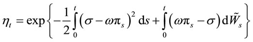
We know that  is a
is a  -Brownian motion, so
  is an
is an  -martingale under measure
 .
.
We have:
Denote that  is an expectation operator with respect to measure
  and let
  is an
is an  -stopping time. Then, by the property
  -martingale under measure
  of
of  (see [4], theorem 11), we have:
 (2.5)
(2.5)
Lemma 1.  can be written as:
 (2.6)
(2.6)
where:  and
and 
Proof.
We have:
and
We consider an optimal stopping problem as:
 (2.7)
(2.7)
where:
where supremum is taken in  -stopping time
  with respect to filtration generated by
  It can be seen that the optimal stopping time in (2.7) can be turned to the optimal stopping time in the problem (2.2).
Now, we study the optimal stopping problem (2.7). We will prove that existing an increasing and continuous monotone function:
such that the stopping time
is an optimal stopping time for the problem (2.7).
 satisfies the equation:
On the other hand, we can write  where
where
With this notation, we have:
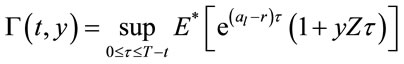
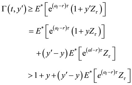
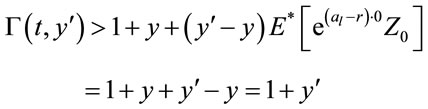
Give  in (2.7), we have

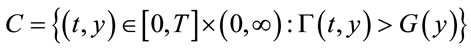
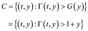
Define the continuation region C:
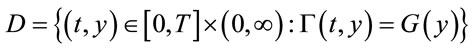
and the stopping region D:
According to general theory about optimal stopping problems, the stopping time
is optimal stopping time problem (2.7). Thus, determining the optimal stopping time is sufficient to defining the stopping region D.
Theorem 1. There exists a right continuous and nondecreasing function
such that
Furthermore, supremum in (7) is achieved with the stopping time
Proof.
We know that
with every fix  and
and , assume that
 , there exists a stopping time
  such that:
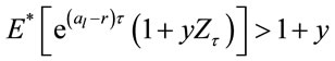
So:
And process  is a submartingale, so we have:
Therefore, . This proves that remaining a function
such that: 
We have  to be a submartingale for
 , so all points in region
 belong to the continuation region.
Therefore, . The monotonicity of b follows from monotonicity of function
 .
.
The right continuity of  follows from the continuation region C is an open set.
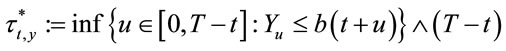
Theorem 2. Assume that b is the function described above whose existence is proved in Lemma 1. Define stopping time:
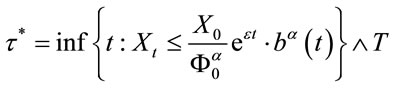 (2.8)
(2.8)
Then,  attains the supremum in (2.2).
Proof. Deduce directly from Theorem 1 and Lemma 1 by replacing  by
by .
.
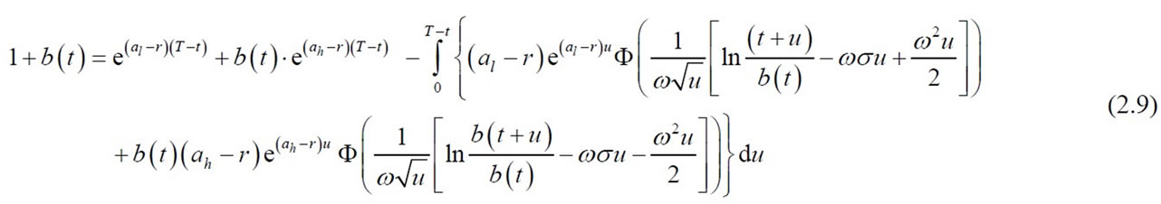
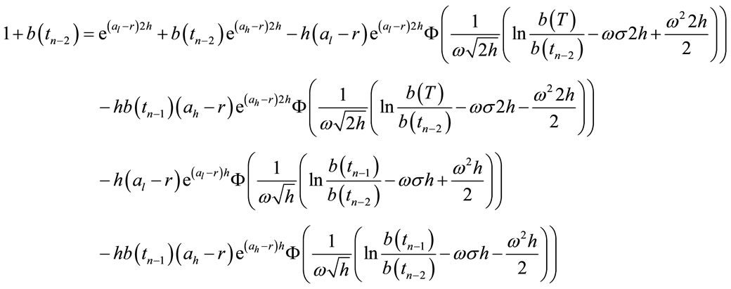
Theorem 3. The optimal stopping boundary b(t) satisfies the integral equation (see Equation (2.9) below):
where 
Proof.
Fix  and
and . Then,
where .
.
But:
Consider:
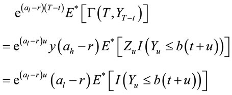
We have:
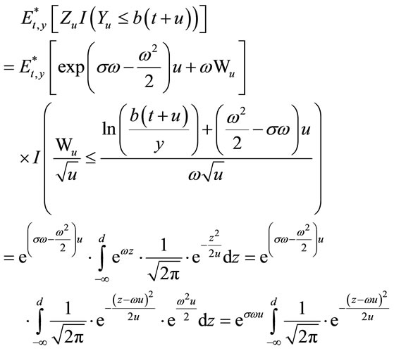
where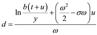 .
.
Let  and
and
then 
In a similar way, we have
where .
.
Put  we attain (2.9).
3. The Numerical Solution of the Integral Equation and Simulation Results
Below we follow [5], devided  by the points
 ,
,  which
which , then Equation (2.8) can be discretized as:
For , we have equation
Due to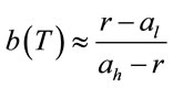 , from the above equation we determine
 , continue to
 , we obtain the following equation for determining
 :
:
Just do so until , it has been determined
 . Thus, we obtain a sequence of values
  of
of  and approximate the optimal boundaries for the asset liquidation process.
We have the approximate solution of Equation (2.9) by a computer program written in Matlab software, then set the boundaries for the process  is
is
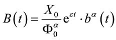 . Then the optimal time to sell is the first time the line describes the process
  lies below the line describes the process
 . These figures (Figures 4-19) and tables below (Tables 1-3) illustrates the stopping time in (2.8) and the solutions of Equation (2.9) in some cases.
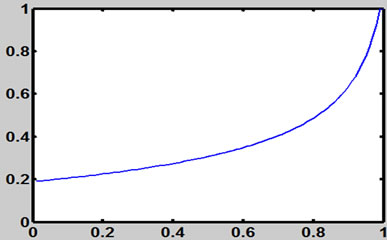
Figure 4. The line describes b (t) with al = 0.1; ah = 0.2; r = 0.15; σ = 0.2.

Figure 5. A simulation for the stopping time in (2.8) with parameters X0 = 3; al = 0.1; ah = 0.2; r = 0.15; σ = 0.2; π0 = 0.5.
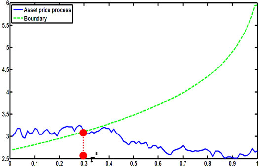
Figure 6. A simulation for the stopping time in (2.8) with parameters X0 = 3; al = 0.1; ah = 0.2; r = 0.15; σ = 0.2; π0 = 0.2. In this case π0 = 0.2 is small so is τ*.
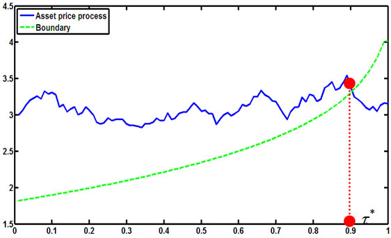
Figure 7. A simulation for the stopping time in (2.8) with parameters X0 = 3; al = 0.1; ah = 0.2; r = 0.15; σ = 0.2; π0 = 0.4.
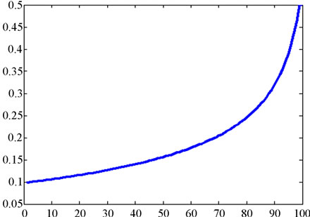
Figure 8. The line describes b (t) with al = 0.09; ah = 0.15; r = 0.11; σ = 0.1.
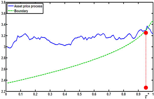
Figure 9. A simulation for the stopping time in (2.8) with parameters X0 = 3; al = 0.09; ah = 0.15; r = 0.11; σ = 0.1; π0 = 0.5.

Figure 10. A simulation for the stopping time in (2.8) with parameters X0 = 3; al = 0.09; ah = 0.15; r = 0.11; σ = 0.1; π0 = 0.4.
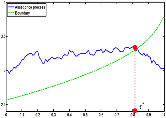
Figure 11. A simulation for the stopping time in (2.8) with parameters X0 = 3; al = 0.09; ah = 0.15; r = 0.11; σ = 0.1; π0 = 0.3.
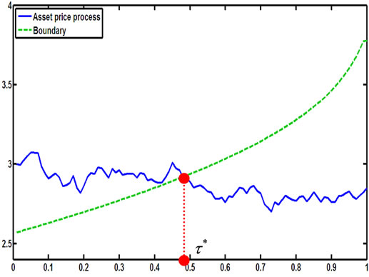
Figure 12. A simulation for the stopping time in (2.8) with parameters X0 = 3; al = 0.09; ah = 0.15; r = 0.11; σ = 0.1; π0 = 0.2.
Figure 13. The line describes b (t) with al = 0.09; ah = 0.15; r = 0.13; σ = 0.1.
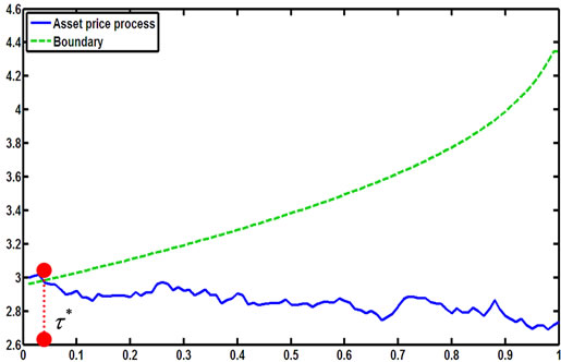
Figure 14. A simulation for the stopping time in (2.8) with parameters X0 = 3; al = 0.09; ah = 0.15; r = 0.13; σ = 0.1; π0 = 0.2.
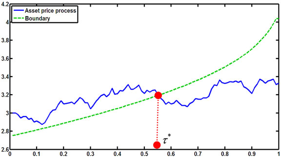
Figure 15. A simulation for the stopping time in (2.8) with parameters X0 = 3; al = 0.09; ah = 0.15; r = 0.13; σ = 0.1; π0 = 0.4.
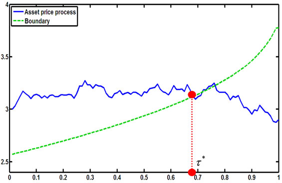
Figure 16. A simulation for the stopping time in (2.8) with parameters X0 = 3; al = 0.09; ah = 0.15; r = 0.13; σ = 0.1; π0 = 0.5.

Figure 17. A simulation for the stopping time in (2.8) with parameters X0 = 3; al = 0.09; ah = 0.15; r = 0.13; σ = 0.1; π0 = 0.5.
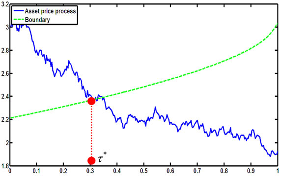
Figure 18. A simulation for the stopping time in (2.8) with parameters X0 = 3; al = –0.3; ah = 0.5; r = 0.1; σ = 0.2; π0 = 0.4.
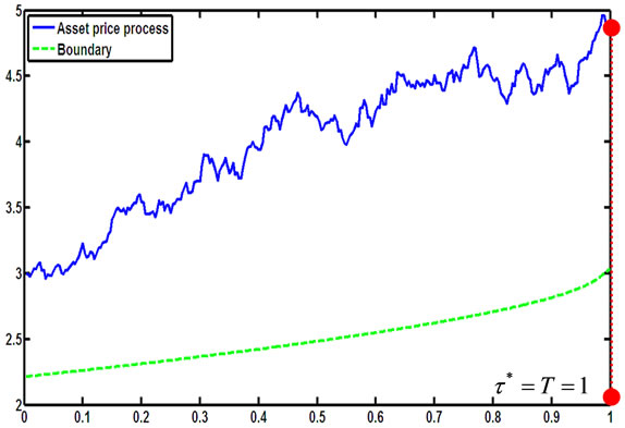
Figure 19. A simulation for the stopping time in (2.9) with parameters X0 = 3; al = –0.3; ah = 0.5; r = 0.1; σ = 0.2; π0 = 0.6.
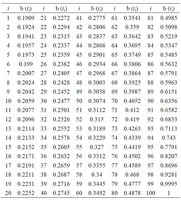
Table 1. The numerical solutions of (2.9) with al = 0.1; ah = 0.2; r = 0.15; σ = 0.2.

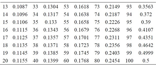
Table 2. The numerical solutions of (2.8) with al = 0.09; ah = 0.15; r = 0.11; σ = 0.1.
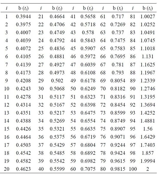
Table 3. The numerical solutions of (2.9) with al = 0.09; ah = 0.15; r = 0.13; σ = 0.1.
4. Conclusion
This paper solves the problem to find the optimal stopping time for the holding asset and make a decision when to sell assets with discounted price reaching the greatest expected value. The optimal stopping time is the first time the price of the asset hit the boundary or be at the time T. In next study, we will study the distributions and characteristics of the optimal stopping time.
REFERENCES
- G. Peskir and A. N. Shiryaev, “Optimal Stopping and Free-Boundary Problems (Lectures in Mathematics ETH Lectures in Mathematics. ETH Zürich (Closed)),” Birkhäuser, Basel, 2006.
- A. N. Shiryaev, Z. Xu and X. Y. Zhou, “Thou Shalt Buy and Hold,” Quantitative Finance, Vol. 8, No. 8, 2008, pp. 765-776.
- R. S. Lipster and A. N. Shiryaev, “Statistics of Random Process: I. General Theory,” Springer-Verlag, Berlin, Heidelberg, 2001.
- A. N. Shiryaev, “Optimal Stopping Rules,” SpringerVerlag, Berlin, Heidelberg, 1978, 2008.
- X. L. Zhang, “Numerical Analysis of American Option Pricing in a Jump-Diffusion Model,” Mathematics of Operations Research, Vol. 22, No. 3, 1997, pp. 668-690. doi:10.1287/moor.22.3.668