Paper Menu >>
Journal Menu >>
 Intelligent Information Management, 2009, 1, 108-119 doi:10.4236/iim.2009.12016 Published Online November 2009 (http://www.scirp.org/journal/iim) Copyright © 2009 SciRes IIM Mediative Fuzzy Logic for Controlling Population Size in Evolutionary Algorithms Oscar MONTIEL1, Oscar CASTILLO2, Patricia MELIN3, Roberto SEPULVEDA4 1,4CITEDI-IPN, Av. del Parque, Mesa de Otay, Tijuana, México 2,3Department of Computer Science, Tijuana Institute of Technology, Chula Vista, USA Email: {oross, rsepulve}@citedi.mx, {ocastillo, pmelin}@tectijuana.mx Abstract: In this paper we are presenting an intelligent method for controlling population size in evolution- ary algorithms. The method uses Mediative Fuzzy Logic for modeling knowledge from experts about what should be the behavior of population size through generations based on the fitness variance and the number of generations that the algorithm is being stuck. Since, it is common that this kind of knowledge expertise can be susceptible to disagreement in a minor or a major part. We selected Mediative Fuzzy Logic (MFL) as a fuzzy method to achieve the inference. MFL is a novelty fuzzy inference method that can handle imperfect knowledge in a broader way than traditional fuzzy logic does. Keywords: mediative fuzzy logic, dynamic population size, HEM 1. Introduction This paper has two mixed goals: one is to present a nov- elty intelligent system for controlling dynamics of popu- lation size in evolutionary algorithms; the second goal is to show an application of mediative fuzzy logic (MFL), a novel fuzzy inference method which is able to handle doubtful and contradictory knowledge, with any degree of mismatch. The goals are mixed because the intelligent system is using MFL to control the population size. In any evolutionary algorithm there are many parame- ters to adjust, and generally they are adjusted by trial and error, one of them is the population size, so it is desirable to have an intelligent evolutionary algorithm, with the capacity of optimizing the population size without the risk of letting the algorithm to get stuck. In real world applications is common that two experts can disagree in some part of the knowledge. Traditional fuzzy logic is unable to handle directly contradiction and hesitation in the knowledge. Uncertainty affects all decision making and appears in a number of different forms. The concept of information is fully connected with the concept of uncertainty; the most fundamental aspect of this connection is that un- certainty involved in any problem-solving situation is a result of some information deficiency, which may be incomplete, imprecise, fragmentary, not fully reliable, vague, contradictory, or deficient in some other way [1]. The general framework of fuzzy reasoning allows han- dling much of this uncertainty. Nowadays, we can handle much of this uncertainty using Fuzzy logic type-1 or type-2 [2,3], also we are able to deal with hesitation using Intuitionistic fuzzy logic in the Atanassov sense, but we have several questions: what happens when the information collected from different sources is somewhat or fully contradictory? What do we have to do if the knowledge base changes with time, and non-contradictory information becomes into doubtful or contradictory information, or any combination of these three situations? What should we infer from this kind of knowledge? The answer to these questions is to use a fuzzy logic system with logic rules for handling non- contradictory, contradictory or information with a hesita- tion margin. Mediative fuzzy logic is a novel approach presented for the first time in [4] which is able to deal with this kind of inconsistent information providing a common sense solution when contradiction exists, this is a mediated solution. There are a lot of applications where information is inconsistent. In economics for estimating the Gross Do- mestic Product (GDP), it is possible to use different variables; some of them are distribution of income, per- sonal consummation expenditures, personal ownership of goods, private investment, unit labor cost, exchange rate, inflation rates, and interest rates. In the same area for estimating the exportation rates it is necessary to use a combination of different variables, for example, the an- nual rate of inflation, the law of supply and demand, the dynamic of international market, etc. [5]. In medicine, information from experiments can be somewhat incon- sistent because living being might respond different to some experimental medication. Currently, randomized clinical trials have become the accepted scientific stan- dard for evaluating therapeutic efficacy, and contradic-  M. MONTIEL ET AL. 109 tory results from multiple randomized clinical trials on the same topic have been attributed either to method- ological deficiencies in the design of one of the trials or to small sample sizes that did not provide assurance that a meaningful therapeutic difference would be detected [6]. In forecasting prediction, uncertainty is always a factor, because to obtain a reliable prediction it is nece- ssary to have a number of decisions, each one based on a different group, in [7] says: Experts should be chosen “whose combined knowledge and expertise reflects the full scope of the problem domain. Heterogeneous experts are preferable to experts focused in a single specialty”. This paper is organized as follows. In Section 2, we are giving some historical antecedent about different logic systems. In Section 3, we are giving a description of the intelligent system for controlling population size in evolutionary algorithms. In Section 4, we are explain- ing concepts of Mediative Fuzzy Logic (MFL). In Sec- tion 5, we are explaining the proposed intelligent system. In Section 6, we are showing results of some experi- ments that we performed. In Section 7, we are making a discussion about the experiment and the obtained results. Finally in Section 8, we are giving the conclusions. 2. Historical Background Throughout history, distinguish good from bad argu- ments has been of fundamental importance to ancient philosophy and modern science. The Greek philosopher Aristotle (384 BC – 322 BC) is considered a pioneer in the study of logic and, its creator in the traditional way. The Organon is his surviving collected works on logic [8]. Aristotelian logic is centered in the syllogism, in Traditional logic, a syllogism (deduction) is an inference that basically consists of three things: the major and minor premises, and the proposition (conclusion) which follows logically from the major and minor premises [9]. Aristotelian logic is “bivalent” or “two-valued”, that is, the semantics rules will assign to every sentence either the value “True” or the value “False”. Two basic laws in this logic are the law of contradiction (p cannot be both p and not p), and the law of the excluded middle (p must be either p or not p). In the Hellenistic period, the stoics work on logic was very wide, but in general, one can say that their logic is based on propositions rather than in logic of terms, like the Aristotelian logic. The Stoic treatment of certain problems about modality and bivalence are more signi- ficant for the shape of Stoicism as a whole. Chrysippus (280BC-206BC) in particular was convinced that biva- lence and the law of excluded middle apply even to contingent statements about particular future events or states of affairs. The law of excluded middle says that for a proposition, p, and its contradictory, ¬p, it is nece- ssarily true, while bivalence insists that the truth table that defines a connective like ‘or’ contains only two values, true and false [10]. In the mid-19th century, with the advent of symbolic logic, we had the next major step in the development of propositional logic with the work of the logicians Au- gustus DeMorgan (1806-1871) [11] and, George Boole (1815-1864). Boole was primarily interested in develop- ing special mathematical to replace Aristotelian syllogis- tic logic. His work rapidly reaps benefits, he proposed “Boolean algebra” that was used to form the basis of the truth-functional propositional logics utilized in computer design and programming [12,13]. In the late 19th century, Gottlob Frege (1848-1925) claimed that all mathematics could be derived from purely logical principles and defi- nitions and he considered verbal concepts to be expressi- ble as symbolic functions with one or more variables [14]. L. E. J. Brouwer (1881-1966) published in 1907 in his doctoral dissertation the fundamentals of intuitionism [15]. His student Arend Heyting (1898-1980) did much to put intuitionism in mathematical logic. He created the Heyting algebra for constructing models of intuitionistic logic [16]. Gerhard Gentzen (1909-1945), in (1934) in- troduces systems of natural deduction for intuitionist and classical pure predicate calculus [17], his cornerstone was cut-elimination theorem which implies that we can put every proof into a (not necessarily unique) normal form. He introduces two formal systems (sequent calculi) LK and LJ. The LJ system is obtained with small changes into the LK system and it is suffice for turning it into a proof system for intuitionistic logic. Nowadays, Intuitionistic logic is a branch of logic which emphasizes that any mathematical object is considered to be a product of a mind, and therefore, the existence of any object is equivalent to the possibility of its construction. This contrasts with the classical app- roach, which states that the existence of an entity can be proved by refuting its non-existence. For the intuitionist, this is invalid; the refutation of the non-existence does not mean that it is possible to find a constructive proof of existence. Intuitionists reject the Law of the Excluded Middle which allows proof by contradiction. Intuitioni- stic logic has come to be of great interest to computer scientists, as it is a constructive logic, and is hence a logic of what computers can do. Bivalent logic was the prevailing view in the development of logic up to XX century. In 1917, Jan Łukasiewicz (1878-1956) developed the three-value pro- positional calculus, inventing ternary logic [18]. His major mathematical work centered on mathematical logic. He thought innovatively about traditional propo- sitional logic, the principle of non-contradiction and the law of excluded middle. Łukasiewicz worked on multi- valued logics, including his own three-valued proposi- tional calculus, the first non-classical logical calculus. He is responsible for one of the most elegant axioma- Copyright © 2009 SciRes IIM  M. MONTIEL ET AL. 110 tizations of classical propositional logic; it has just three axioms and is one of the most used axiomatizations today [19]. Paraconsistent logic is a logic rejecting the principle of non-contradiction, a logic is said to be paraconsistent if its relation of logical consequence is not explosive. The first paraconsistent calculi was independently proposed by Newton C. da Costa (1929- ) [20] and Jaśkowski, and are also related to D. Nelson’s ideas [21]. Paraconsistent logic was proposed in 1976 by the Peruvian philosopher Miró Quesada, it is a non-trivial logic which allows in- consistencies. The modern history of paraconsistent logic is relatively short. The expression “paraconsistent logic” is at present time well-established and it will make no sense to change it. It can be interpreted in many different ways which correspond to the many different views on a logic which permits to reason in presence of contradic- tions. There are many different paraconsistent logics, for example, non-adjunctive, non-truth-functional, many- valued, and relevant. Fuzzy sets, and the notions of inclusion, union, intersection, relation, etc, were introduced in 1965 by Dr. Lofti Zadeh [2], as an extension of Boolean logic. Fuzzy logic deals with the concept of partial truth, in other words, the truth values used in Boolean logic are replaced with degrees of truth. Zadeh is the creator of the concept Fuzzy logic type-1 and type-2. Type-2 fuzzy sets are fuzzy sets whose membership functions are them- selves type-1 fuzzy sets; they are very useful in circum- stances where it is difficult to determine an exact mem- bership function for a fuzzy set [22]. K. Atanassov in 1983 proposed the concept of Intui- tionistic fuzzy sets (IFS) [23], as an extension of the well-known Fuzzy sets defined by Zadeh. IFS introduces a new component, degree of non-membership with the requirement that the sum of membership and non-mem- bership functions must be less than or equal to 1. The complement of the two degrees to 1 is called the hesi- tation margin. George Gargov proposed the name of intuitionistic fuzzy sets with the motivation that their fuzzification denies the law of excluded middle, wish is one of the main ideas of intuitionism [24]. 3. Intelligent System Description In Figure 1, we are showing in general terms a method for controlling population size in evolutionary algorithms. This is an intelligent system that adapts the population size according to some predefined behavioral rules. We used MFL to achieve the inference, we selected this method because it can handle doubtful and contradictory knowledge provided by human experts, and moreover, the method is auto-reducible, so if there is no contra- diction or hesitation in the knowledge, the system will behaves as a traditional fuzzy inference system. Basically, the method is using two variables, the variance in the fitness value of the best individual in previous generations; and the degree of cycling that the algorithm is having. In order to calculate the variance, we considered the last ten generations to perform the calculation. The degree of cycling is a way to measure how many generations has passed without any significant change in the variance measure. This method can be applied practically to any evolutionary algorithm, in our case we used the Human Evolutionary Model (HEM) since this method was designed originally to be used with this evolutionary method. In Figure 1, we can appreciate in the first five lines that they are devote to the method initialization, here N is the initial population size; in the evolution process, we can vary this population between an upper and lower bound (ub, and lb). The evolutionary algorithm will run “maxGen” number of generations, Figure 1. Generic method for controlling population size using the variance of the fitness and the degree of cycling; i.e. the number of generations that the algorithms has ran without any significant change in the fitness value Copyright © 2009 SciRes IIM  M. MONTIEL ET AL. 111 Figure 2. Inference system at the agreement side. Here, the system is defined using the agreement MFs Figure 3. Inference system at the non-agreement side. The system is defined using the non-agreement MFs although we can change this condition to a specific accuracy value. Next, the selected evolutionary algorithm will run one gener- ation at each cycle, after that we will measure the variance and degree of cycling that the algorithm is having. To measure the cyclyng we are using the variable “Cycling”, an increment in this variable is done every time that the variance in the fitness is below a determined threshold value (0.05 in this case), otherwise the variable is reset. The intelligent system will calculate the amount of individuals to delete and to create using the inference system based in MFL, this action is expressed in Figure 1 by means of the function “calculate_aiis_hem”. This function has two input parameters, they are “Cycling” and “Variance”; and the output “y_aiis” is a vector with two values, they are proportional indexes. The valid range of each index is [0,1]. Hence, the amount of individuals to create is calculated using the formula of line 16, and the amount of individuals to delete using the formula of line 17. Next, the algorithm goes into a process of deleting the worst (less fit) individual in the actual population expressed by the variable “Delete”, then we will create an amount of individuals expressed by the variable “Create”. Both processes are controlled to be into a valid range delimited by the upper and lower bound in the population size. 4. Mediative Fuzzy Logic Since knowledge provided by experts can have big varia- tions and sometimes can be contradictory, we are pro- posing to use a Contradiction fuzzy set to calculate a mediation value for solving the conflict. Mediative Fuzzy Logic is proposed as an extension of traditional fuzzy logic and includes Intuistionistic Fuzzy Logic (IFL) in the Atanassov sense [23,25]. Hence, it is able to handle contradictory and doubtful information. A traditional fuzzy set in X [25], is given by A = {(x, A(x))| x X} (1) where A : X [0, 1] is the membership function of the fuzzy set A. An IFL set B is given by XxxxxB BB |,, (2) where B : X [0, 1] and B : X [0, 1] are such that 10 xx BB (3) and B(x); B(x) [0, 1] denote a degree of membership and a degree of non-membership of x A, respectively. For each IFL set in X we have a “hesitation margin” x B , this is a fuzzy index of x B, it expresses a hesitation degree of whether x belongs to A or not. It is obvious that 10 x B , for each . Xx xxx BBB 1 (4) Therefore if we want to fully describe an IFL set, we must use any two functions from the triplet [10]. 1) Membership function 2) Non-membership function 3) Hesitation margin The application of IFL sets instead of fuzzy sets, means the introduction of another degree of freedom into a set description, in other words, in addition to B we also have B or B . IFL considers the fact that we have the membership functions as well as the non-membership functions . Hence, the output of an IFL system can be calculated as follows: FSFSIFS 1 (5) Copyright © 2009 SciRes IIM  M. MONTIEL ET AL. 112 where F S is the traditional output of a fuzzy system using the membership function , and is the out- put of a fuzzy system using the non-membership func- tion FS . Note in Equation (6), when =0 the IFS is reduced to the output of a traditional fuzzy system, but if we take into account the hesitation margin of the re- sulting IFS will be different. In similar way, a contradiction fuzzy set C in X is given by: xxx CCC ,min (6) where C x represents the agreement membership function, and for the variable x C we have the non-agreement membership function. We are using the agreement and non-agreement in- stead membership and non-membership, because we think these names are more adequated when we have contradictory fuzzy sets. For calculating the inference at the system’s output, we are using FSFSMFS 22 1 (7) 5. Defining the Intelligent System We used MFL to control the population size of HEM by killing and/or creating individuals in the new population. A Sugeno Inference System at the agreement side (AIISa) was used to calculate the fuzzy outputs Create and Delete. In the same way, at the non-Agreement side (AIISna) we have the fuzzy outputs Create and Delete. See in Figures 4 and 5 a block diagram of both inference systems. For both inference systems, we defined two linguistic input variables: Cycling and Variance. The variable Cycling is representing the amount of generations that has passed with any significative change in the variance value of the fitness over a Figure 4. Inference system at the agreement side. Here, the system is defined using the agreement MFs Figure 5. Inference system at the non-agreement side. The system is defined using the non-agreement MFs Figure 6. MFs for the variable Cycling at the agreement side in a traditional fuzzy system. Figure 7. MFs for the variable Cycling a the non-agreement side Copyright © 2009 SciRes IIM  M. MONTIEL ET AL. Copyright © 2009 SciRes IIM 113 determined number of generations. The variable Variance is calculated using the actual and past values of the population’s fitness. We used the fitness value obtained in the last ten generations (including the actual generation). For taking into account an increment in the variable Cycling, we used a threshold variance value of 0.05, any value below the threshold increases the Cycling counter, otherwise the variable Cycling must be reset. At the agreement side, the input variables Cycling has four terms: SmallC, RegularC, LargeC, XLargeC; see Figure 6. The input variable Variance has four terms: SmallV, RegularV, LargeV, XLargeV, see Figure 8. At the non-agreement side, the input variable Cycling has two terms: nLargeC, nSmallC; see Figure 7. The input variable Variance also has two terms: nLargeV, nSmallV, see Figure 9. In Table 1, we are summarizing the the names, type and parameters for each input variable. Each Inference fuzzy system has two output variables: Delete and Create. They correspond to the amount of individuals that we have to delete in the actual popula- tion, and to create in the new population. Each output variable has three constant terms: little, regular and many. We used the same constant term names and values for every term at each output of both Sugeno type 0 infer- ence systems. We assigned the values of “0”, “0.5”, and “1” to the variables little, regular and many, respectively. At the agreement side we have the next fuzzy rules: 1. If (Cyicling is SmallC) and (Variace is SmallV) then (Create is little)(Delete is little) 2. If (Cyicling is SmallC) and (Variace is RegularV) then (Create is regular)(Delete is little) 3. If (Cyicling is SmallC) and (Variace is LargeV) then (Create is regular)(Delete is regular) 4. If (Cyicling is RegularC) and (Variace is SmallV) then (Create is many)(Delete is regular) 5. If (Cyicling is RegularC) and (Variace is RegularV) then (Create is regular)(Delete is regular) 6. If (Cyicling is RegularC) and (Variace is LargeV) then (Create is regular)(Delete is regular) 7. If (Cyicling is LargeC) and (Variace is SmallV) then (Create is many)(Delete is many) 8. If (Cyicling is LargeC) and (Variace is RegularV) then (Create is many)(Delete is regular) 9. If (Cyicling is LargeC) and (Variace is LargeV) then (Create is little)(Delete is little) 10. If (Cyicling is SmallC) and (Variace is XLargeV) then (Create is little)(Delete is regular) 11. If (Cyicling is RegularC) and (Variace is XLargeV) then (Create is regular)(Delete is little) 12. If (Cyicling is LargeC) and (Variace is XLargeV) then (Create is little)(Delete is little) 13. If (Cyicling is XLargeC) and (Variace is SmallV) then (Create is many)(Delete is many) 14. If (Cyicling is XLargeC) and (Variace is RegularV) then (Create is many)(Delete is many) 15. If (Cyicling is XLargeC) and (Variace is XLargeV) then (Create is many)(Delete is many) 16. If (Cyicling is XLargeC) and (Variace is LargeV) then (Create is many)(Delete is many) Table 1. Linguistic input variables for the fuzzy system at the agreement side (AIISa), and for fuzzy system at the non-agreement side AIISna FIS name Variable name Term name Type Parameters AIISa ( F S ) Cycling SmallC Trapezoidal [-1,-1,5,30] AIISa( F S ) Cycling RegularC Triangular [10,30,50] AIISa ( F S ) Cycling LargeC Triangular [30,50,70] AIISa ( F S ) Cycling XLargeC Trapezoidal [50,70,5e+15,5e+15] AIISa ( F S ) Variance SmallV Trapezoidal [-1,-1,0.04,0.2] AIISa ( F S ) Variance RegularV Triangular [0,0.2,0.4] AIISa ( F S ) Variance LargeV Triangular [0.2,0.4,0.6] AIISa ( F S ) Variance XLargeV Trapezoidal [0.4,0.6,5e+15,5e+15] AIISna ( F S ) Cycling nLargeC Trapezoidal [-1,-1,10,60] AIISna ( F S ) Cycling nSmallC Trapezoidal [10,60,5e+15,5e+15] AIISna ( F S ) Variance nLargeV Trapezoidal [-1,-1,0.05,1] AIISna ( F S ) Variance nSmallV Trapezoidal [-1,0.09,1,5e+15]  M. MONTIEL ET AL. 114 At the non-agreement side, we have the next fuzzy rules: 1. If (Cyicling is nLargeC) and (Variance is nLargeV) then (Create is little)(Delete is little) 2. If (Cyicling is nLargeC) and (Variance is nSmallV) then (Create is little)(Delete is little) 3. If (Cyicling is nSmallC) and (Variance is nLargeV) then (Create is many)(Delete is many) 4. If (Cyicling is nSmallC) and (Variance is nSmallV) then (Create is regular)(Delete is regular) 6. Experiments For Experiments 1 and 2, we ran the evolutionary algo- rithm 1500 generations with the purpose of analyzing the dynamic behavior of the population size. We used an ini- tial population size of 100 individuals, the selected upper and lower bounds (ub and lb) to control population size within a range were 600 and 20 individuals respectively. In Experiment 3, we only changed the initial popula- tion size to 20. 6.1. Experiment #1. 4-Dimensions Rosenbrock Function The Rosenbroc function is given by Equation (7). This function has its minimal value at . After 1500 generations we found the value , and the corresponding fitness value is 9.08, it last 31 seconds. Figure 22 shows the fitness behavior and Figure 23 shows how the size of population is changing in order to help the algorithm to obtain an increment in the overall fitness. 1,1,1,1 *x 51.0,72.0,85.0,92.0 *x 1 1 2 2 2 11*1002 N i iii xxxxF (7) 6.2. Experiment #2. 4-Dimensions Rastrigin Function The Rastriging function is given by Equation (8). This function has its minimal in. After 1500 generations we found a fitness values around 1.16 × 10⁹, in this example the minimal value founded is in 0,0,0,0 *x 55 103.0,10 5* 2.0,10049.0,0.0 x. The algo- rithm last 33.8 seconds, but in fact the algorithm is able to find values with very high fitness more or less in 20 generations. In Figure 24, we are showing the fitness evolution through 1500 generations. In the Rastrigin function, n is the dimension of the problem, and the variables A and w control the ampli- tude and frequency modulation respectively. n i iixwAxnAxF 1 2cos (8) 6.3. Experiment #3. 4-Dimension Rastrigin Function In Figure 24 we are showing a second run, here we used 20 generations, and the other test conditions were the same. In this case, the algorithm last 0.5540 seconds, and the values found were , with a fitness value of 26.03. ,0062.0,0117.0[ *x ]0040.0,0014.0 7. Discussion The agreement membership functions and the non- agreement membership functions were collected from two different experts. It was easier to define the agree- Figure 8. MFs for the variable variance at the agreement side Figure 9. MFs for the variable variance at the non-agre ement side Copyright © 2009 SciRes IIM  M. MONTIEL ET AL. 115 Figure 10. Hesitation fuzzy set for the variable cycling Figure 11. Contradiction fuzzy set for the variable cycling Figure 12. Hesitation fuzzy set for the variable variance Figure13. Contradiction fuzzy set for the variable variance Figure 14. Surface of the fuzzy output create at the agree- ment side of a traditional fuzzy system Figure 15. Surface of the mediated fuzzy output create Copyright © 2009 SciRes IIM  M. MONTIEL ET AL. 116 Figure 16. Surface of the fuzzy output create at the non-ag- reement side Figure 17. Surface of the mediated fuzzy output delete Figure 18. Surface of the variable delete at the agreement side in a traditional fuzzy system Figure 19. Surface of the mediated fuzzy output delete Figure 20. This fitness plot was obtained as a result of find- ing the minimizers for the 4-D Rosenbrock function. Ex- periment 1 Figure 21. Dynamical behavior of population when the evolutionary algorithm is finding the function’s minimizers. Experiment 1 Copyright © 2009 SciRes IIM 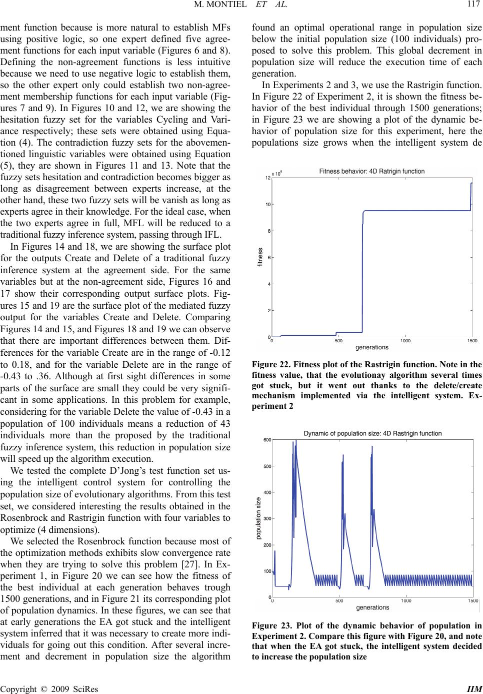 M. MONTIEL ET AL. 117 ment function because is more natural to establish MFs using positive logic, so one expert defined five agree- ment functions for each input variable (Figures 6 and 8). Defining the non-agreement functions is less intuitive because we need to use negative logic to establish them, so the other expert only could establish two non-agree- ment membership functions for each input variable (Fig- ures 7 and 9). In Figures 10 and 12, we are showing the hesitation fuzzy set for the variables Cycling and Vari- ance respectively; these sets were obtained using Equa- tion (4). The contradiction fuzzy sets for the abovemen- tioned linguistic variables were obtained using Equation (5), they are shown in Figures 11 and 13. Note that the fuzzy sets hesitation and contradiction becomes bigger as long as disagreement between experts increase, at the other hand, these two fuzzy sets will be vanish as long as experts agree in their knowledge. For the ideal case, when the two experts agree in full, MFL will be reduced to a traditional fuzzy inference system, passing through IFL. In Figures 14 and 18, we are showing the surface plot for the outputs Create and Delete of a traditional fuzzy inference system at the agreement side. For the same variables but at the non-agreement side, Figures 16 and 17 show their corresponding output surface plots. Fig- ures 15 and 19 are the surface plot of the mediated fuzzy output for the variables Create and Delete. Comparing Figures 14 and 15, and Figures 18 and 19 we can observe that there are important differences between them. Dif- ferences for the variable Create are in the range of -0.12 to 0.18, and for the variable Delete are in the range of -0.43 to .36. Although at first sight differences in some parts of the surface are small they could be very signifi- cant in some applications. In this problem for example, considering for the variable Delete the value of -0.43 in a population of 100 individuals means a reduction of 43 individuals more than the proposed by the traditional fuzzy inference system, this reduction in population size will speed up the algorithm execution. We tested the complete D’Jong’s test function set us- ing the intelligent control system for controlling the population size of evolutionary algorithms. From this test set, we considered interesting the results obtained in the Rosenbrock and Rastrigin function with four variables to optimize (4 dimensions). We selected the Rosenbrock function because most of the optimization methods exhibits slow convergence rate when they are trying to solve this problem [27]. In Ex- periment 1, in Figure 20 we can see how the fitness of the best individual at each generation behaves trough 1500 generations, and in Figure 21 its corresponding plot of population dynamics. In these figures, we can see that at early generations the EA got stuck and the intelligent system inferred that it was necessary to create more indi- viduals for going out this condition. After several incre- ment and decrement in population size the algorithm found an optimal operational range in population size below the initial population size (100 individuals) pro- posed to solve this problem. This global decrement in population size will reduce the execution time of each generation. In Experiments 2 and 3, we use the Rastrigin function. In Figure 22 of Experiment 2, it is shown the fitness be- havior of the best individual through 1500 generations; in Figure 23 we are showing a plot of the dynamic be- havior of population size for this experiment, here the populations size grows when the intelligent system de Figure 22. Fitness plot of the Rastrigin function. Note in the fitness value, that the evolutionay algorithm several times got stuck, but it went out thanks to the delete/create mechanism implemented via the intelligent system. Ex- periment 2 Figure 23. Plot of the dynamic behavior of population in Experiment 2. Compare this figure with Figure 20, and note that when the EA got stuck, the intelligent system decided to increase the population size Copyright © 2009 SciRes IIM 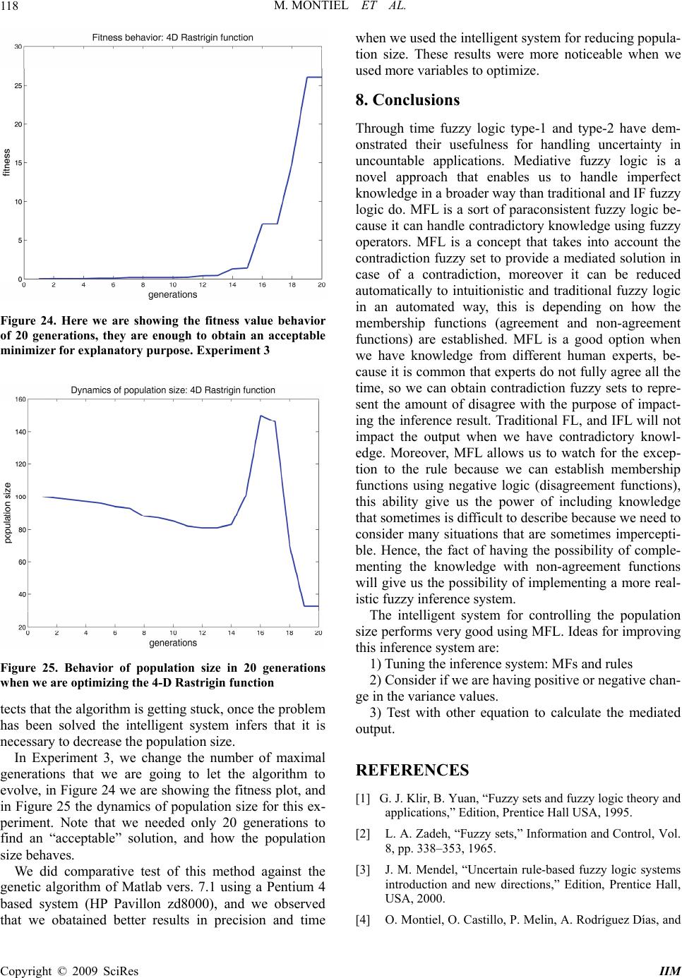 M. MONTIEL ET AL. 118 Figure 24. Here we are showing the fitness value behavior of 20 generations, they are enough to obtain an acceptable minimizer for explanatory purpose. Experiment 3 Figure 25. Behavior of population size in 20 generations when we are optimizing the 4-D Rastrigin function tects that the algorithm is getting stuck, once the problem has been solved the intelligent system infers that it is necessary to decrease the population size. In Experiment 3, we change the number of maximal generations that we are going to let the algorithm to evolve, in Figure 24 we are showing the fitness plot, and in Figure 25 the dynamics of population size for this ex- periment. Note that we needed only 20 generations to find an “acceptable” solution, and how the population size behaves. We did comparative test of this method against the genetic algorithm of Matlab vers. 7.1 using a Pentium 4 based system (HP Pavillon zd8000), and we observed that we obatained better results in precision and time when we used the intelligent system for reducing popula- tion size. These results were more noticeable when we used more variables to optimize. 8. Conclusions Through time fuzzy logic type-1 and type-2 have dem- onstrated their usefulness for handling uncertainty in uncountable applications. Mediative fuzzy logic is a novel approach that enables us to handle imperfect knowledge in a broader way than traditional and IF fuzzy logic do. MFL is a sort of paraconsistent fuzzy logic be- cause it can handle contradictory knowledge using fuzzy operators. MFL is a concept that takes into account the contradiction fuzzy set to provide a mediated solution in case of a contradiction, moreover it can be reduced automatically to intuitionistic and traditional fuzzy logic in an automated way, this is depending on how the membership functions (agreement and non-agreement functions) are established. MFL is a good option when we have knowledge from different human experts, be- cause it is common that experts do not fully agree all the time, so we can obtain contradiction fuzzy sets to repre- sent the amount of disagree with the purpose of impact- ing the inference result. Traditional FL, and IFL will not impact the output when we have contradictory knowl- edge. Moreover, MFL allows us to watch for the excep- tion to the rule because we can establish membership functions using negative logic (disagreement functions), this ability give us the power of including knowledge that sometimes is difficult to describe because we need to consider many situations that are sometimes impercepti- ble. Hence, the fact of having the possibility of comple- menting the knowledge with non-agreement functions will give us the possibility of implementing a more real- istic fuzzy inference system. The intelligent system for controlling the population size performs very good using MFL. Ideas for improving this inference system are: 1) Tuning the inference system: MFs and rules 2) Consider if we are having positive or negative chan- ge in the variance values. 3) Test with other equation to calculate the mediated output. REFERENCES [1] G. J. Klir, B. Yuan, “Fuzzy sets and fuzzy logic theory and applications,” Edition, Prentice Hall USA, 1995. [2] L. A. Zadeh, “Fuzzy sets,” Information and Control, Vol. 8, pp. 338–353, 1965. [3] J. M. Mendel, “Uncertain rule-based fuzzy logic systems introduction and new directions,” Edition, Prentice Hall, USA, 2000. [4] O. Montiel, O. Castillo, P. Melin, A. Rodríguez Días, and Copyright © 2009 SciRes IIM  M. MONTIEL ET AL. Copyright © 2009 SciRes IIM 119 R. Sepúlveda, ICAI, 2005. [5] D. A. Bal, and W. H. McCulloch, Jr., “International business introduction and essentials,” Fifth Edition, pp. 138–140, 225, USA, 1993. [6] R. I. Horwitz, “Complexity and contradiction in clinical trial research,” American Journal of Medicine, Vol. 8, pp. 498–510, 1987. [7] J. S. Armstrong, “Principles of forecasting, A handbook for researchers and practitioners,” Edited by J. Scott Armstrong, University of University of Pennsylvania, Wharton School, Philadelphia, PA., USA, 2001. [8] Aristotle, “The basic works of Aristotle,” Modern Library Classics, Richard McKeon Edition, 2001. [9] R. Smith, “Aristotle’s logic, Stanford encyclopedia of philosophy,” 2004. http://plato.stanford.edu/entries/aris- totle-logic/. [10] D. Baltzly, “Stanford encyclopedia of philosophy,” 2004. http://plato.stanford.edu/entries/stoicism/. [11] J. J. O’Connor E. F. Robertson, and A. DeMorgan, “Mac- Tutor history of mathematics: Indexes of biographies (University of St. Andrews),” 2004, http://www-groups. dcs.st-andrews.ac.uk/~history/Mathematicians/De_Morga n.htm. [12] G. Boole, “The calculus of logic,” Cambridge and Dublin Mathematical Journal, Vol. 3, pp. 183–98, 1848. [13] J. J. O’Connor, E. F. Robertson, G. Boole, and MacTutor history of mathematics: Indexes of biographies,” Univer- sity of St. Andrews, 2004. http://www-groups.dcs.st-an- drews.ac.uk/~history/Mathematicians/Boole.html. [14] J. J. O’Connor, E. F. Robertson, F. L. G. Frege, and Mac Tutor history of mathematics: Indexes of Biographies University of St. Andrews, http://www-groups.dcs.st-an- drews.ac.uk/~history/Mathematicians/Frege.html. [15] J. J. O’Connor and E. F. Robertson , L. E. J. Brouwer, MacTutor history of mathematics: Indexes of biogra- phies,” University of St. Andrews, http://www-groups.dcs. st-adrews.ac.uk/~history/Mathematicians/Brouwer.html. [16] J. J. O’Connor, E. F. Robertson, and A. Heyting, “Mac- Tutor history of mathematics: Indexes of biographies,” University of St. Andrews, 2004. http://www-history. mcs.st-adrews.ac.uk/Mathematicians/Heyting.html. [17] J. J. O’Connor, E. F. Robertson, and G. Gentzen, “Mac- Tutor history of mathematics: Indexes of biographies,” University of St. Andrews, 2004. http://www-history. mcs.st-andrews.ac.uk/Mathematicians/Gentzen.html. [18] J. J. O’Connor, E. F. Robertson, and J. Lukasiewicz, “MacTutor history of mathematics: Indexes of biogra- phies,” University of St. Andrews, 2004. http://www-his- tory.mcs.st-andrews.ac.uk/Mathematicians/Lukasiewicz.h tml. [19] Wikipedia the free encyclopedia, http://en.wikipedia.org/ wiki/Jan_Lukasiewicz. [20] Wikipedia the free encyclopedia, http://en.wikipedia.org/ wiki/Newton_da_Costa. [21] W. A. Carnielli, “How to build your own paraconsistent logic: An introduction to the logics of formal (in) consis- tency,” In: J. Marcos, D. Batens, and W. A. Carnielli, or- ganizers, Proceedings of the Workshop on Paraconsistent Logic (WoPaLo), held in Trento, Italy, as part of the 14th European Summer School on Logic, Language and In- formation (ESSLLI’02), pp. 58–72, 5–9 August 2002. [22] J. M. Mendel and R. B. John, “Type-2 fuzzy sets made simple,” IEEE Transactions on Fuzzy Systems, Vol. 10, No. 2, April 2002. [23] K. Atanassov, “Intuitionistic guzzy dets: Theory and spplications,” Springer-Verlag, Heidelberg, Germany, 1999. [24] M. Nikilova, N. Nikolov, C. Cornelis, and G. Deschri- jver, “Survey of the research on intuitionistic fuzzy sets,” In: Advanced Studies in Contemporary Mathematics, Vol. 4, No. 2, , pp. 127–157, 2002. [25] C. P. Melin, “A new method for fuzzy inference in in- tuitionistic fuzzy systems, proceedings of the interna- tional conference,” NAFIPS’03, IEEE Press, Chicago, Il- linois, USA, Julio, pp. 20–25, 2003. [26] O. Nelles, “Nonlinear system identification from classical approaches to neural networks and fuzzy models,” Springer-Verlag, Germany, 2001. |