Intelligent Information Management, 2009, 1, 98-107
doi:10.4236/iim.2009.12015 Published Online November 2009 (http://www.scirp.org/journal/iim)
What can Software Engineers Learn from
Manufacturing to Improve Software Process
and Product?
Norman SCHNEIDEWIND
Information Sciences, Naval Postgraduate School, Monterey, US
Abstract: The purpose of this paper is to provide the software engineer with tools from the field of manu-
facturing as an aid to improving software process and product quality. Process involves classical manufactur-
ing methods, such as statistical quality control applied to product testing, which is designed to monitor and
correct the process when the process yields product quality that fails to meet specifications. Product quality is
measured by metrics, such as failure count occurring on software during testing. When the process and prod-
uct quality are out of control, we show what remedial action to take to bring both the process and product
under control. NASA Space Shuttle failure data are used to illustrate the process methods.
Keywords: manufacturing methods, software process, software product, product and process quality, Taguchi
methods
1. Introduction
Based on “old” ideas from the field of manufacturing, we
propose “new” ideas for software practitioners to con-
sider for controlling the quality of software. Although
there are obviously significant difference between hard-
ware and software, there are design quality control proc-
esses that can be adapted from hardware and applied
advantageously to software. Among these are the Ta-
guchi manufacturing methods, statistical quality control
charts (statistical quality control is the use of statistical
methods to control quality [1]), and design of experi-
ments. These methods assess whether a product manu-
facturing process is within statistical control. Statistical
control means that product attributes like software failure
occurrence is within specified control limits.
Every process has inherent variation that hampers ac-
curate process prediction. In addition, interactions of
people, machines, environment, and methods introduce
noise into the system. You can control the inherent varia-
tion by identifying and controlling its cause, thereby
bringing the process under statistical control [2]. While
this is important, we should not get carried away by fo-
cusing exclusively on process. Most customers do not
care about process. They are interested in product quality!
Thus, when evaluating process improvement, it is crucial
to measure it in terms of the product quality that is
achieved. Thus, we explore methods, like Taguchi meth-
ods, that tie process to product. We apply these methods
to NASA Space Shuttle software using actual failure data.
The use of the Shuttle as an example is appropriate be-
cause this is a CMMI Level 5 process that uses product
quality measurements to improve the software develop-
ment process [3]. It is a characteristic of processes at this
level that the focus is on continually improving process
performance through both incremental and innovative
technological changes and improvements. At maturity
level 5, processes are concerned with addressing statisti-
cal common causes of process variation and changing the
process (for example, shifting the mean of the process
performance) to improve process performance. This
would be done at the same time as maintaining the like-
lihood of achieving the established quantitative process-
improvement objectives. While some software engineers
argue that a CMMI Level 5 process is not applicable to
their software, we suggest that it is applicable to any
software as an objective, with the benefit of evolving to a
higher CMMI level.
Typical metrics that software engineers use for assess-
ing software quality are defect, fault, and failure counts,
complexity measures that measure the intricacies of the
program code, and software reliability prediction models.
The data to drive these methods are collected from defect
reports, code inspections, and failure reports. The data
are collected either by software engineers or automati-
cally by using a variety of software measurement tools.
These data are used in design and code inspections to
remove defects and in testing to correct faults.
Since software engineers are typically not schooled in

N. SCHNEIDEWIND
99
manufacturing systems, they are unaware of how manu-
facturing methods can be applied to improving the qual-
ity of software. Our objective is to show software re-
searchers and practitioners how manufacturing methods
can be applied to improving the quality of software.
2. Relationship of Manufacturing to
Software Development
There is a greater intersection between manufacturing
methods and software development than software practi-
tioners realize. For example, software researchers and
industry visionaries have long dreamed about a Leg0
block style of software development: building systems
by assembling prefabricated, ready-to-use parts. Over the
last several decades, we have seen the focus of software
development shift from the generation of individual pro-
grams to the assembly of large number of components
into systems or families of systems. The two central
themes that emerged from this shift are components, the
basic system building blocks, and architectures, the de-
scriptions of how components are assembled into sys-
tems. Interest in components and architectures has gone
beyond the research community in recent years. Their
importance has increasingly been recognized in industry.
Today, a business system can be so complex that major
components must be developed separately. Nevertheless,
these individually developed components must work
together when the system is integrated. The need for a
component-based strategy also arises from the increased
flexibility that businesses demand of themselves and, by
extension, of their software systems. To address the
business needs, the software industry has been moving
very rapidly in defining architecture standards and de-
veloping component technologies. An emerging trend in
this movement has been the use of middleware, a layer of
software that insulates application software from system
software and other technical or proprietary aspects of
underlying run-time environments. [4] Component-based
software construction enhances quality by confining
faults and failures to specific components so that the
cause of the problem can be isolated and the faults re-
moved.
Manufacturing is an important part of any software
development process. In the simplest case, a single
source code file must be compiled and linked with sys-
tem libraries. More usually, a program will consist of
multiple separately written components. A program of
this kind can be manufactured by compiling each com-
ponent in turn and then linking the resulting object mod-
ules. Software generators introduce more complexity into
the manufacturing process. When using a generator, the
programmer specifies the desired effect of a component
and the generator produces the component implementa-
tion. Generators enable effective reuse of high-level de-
signs and software architectures. They can embody state
of-the-art implementation methods that can evolve with-
out affecting what the programmer has to write. While
the programmer can manually invoke compilers and
linkers, it is much more desirable to automate the soft-
ware manufacturing process. The main advantage of
automation is that it ensures manufacturing steps are
performed when required and that only necessary steps
are performed. These benefits are particularly noticeable
during maintenance of large programs, perhaps involving
multiple developers. Automation also enables other par-
ties to manufacture the software without any detailed
knowledge of the process. [5] Component reuse is a boon
to software reliability because once a component is de-
bugged, it can be used repeatedly with assurance that it is
reliable.
Another tool borrowed from manufacturing is con-
figuration control [6]. At first blush, one may wonder
how configuration control fits with software develop-
ment. Actually, it is extremely important because soft-
ware is subject to change throughout the life cycle in
requirements, design, coding, testing, operation and
maintenance. A dramatic illustration of the validity of
this assertion is the software maintenance function. For
example, no sooner is the software delivered to the cus-
tomer than requests for changes are received by the de-
veloper. This is in addition to the changes caused by bug
fixes after delivery. If configuration management is not
employed, the process will become chaotic with neither
customer nor developer knowing the state of the software
and the status of the process.
3. Arguments against Applying
Manufacturing Methods to Software
We note that not all software engineers subscribe to the
idea that manufacturing methods can be applied to soft-
ware. They claim that it is infeasible to measure software
because unlike high volume manufacturing of hardware,
with close tolerances, many software projects are low
volume produced with a fuzzy process, where product
tolerance has no meaning. [7] Actually, none of this is
true. While component-based software development is
not a high volume process, it produces products for use
in a large number of applications (e.g., edit module in a
word processor). As for process, we have cited the
CMMI Level 5 process that can control the variation in
product quality by feeding back deviations in product
quality to the development process for the purpose of
correction the process that led to undesired variance in
product quality. While it is true that software cannot be
manufactured to the precision of software, statistical
quality control of defect count, confidence intervals of
reliability predictions, numerical reliability specifications,
and quality prediction accuracy measurement, are just a
few of the quantitative measurements from the physical
world that have been applied to software, for example, in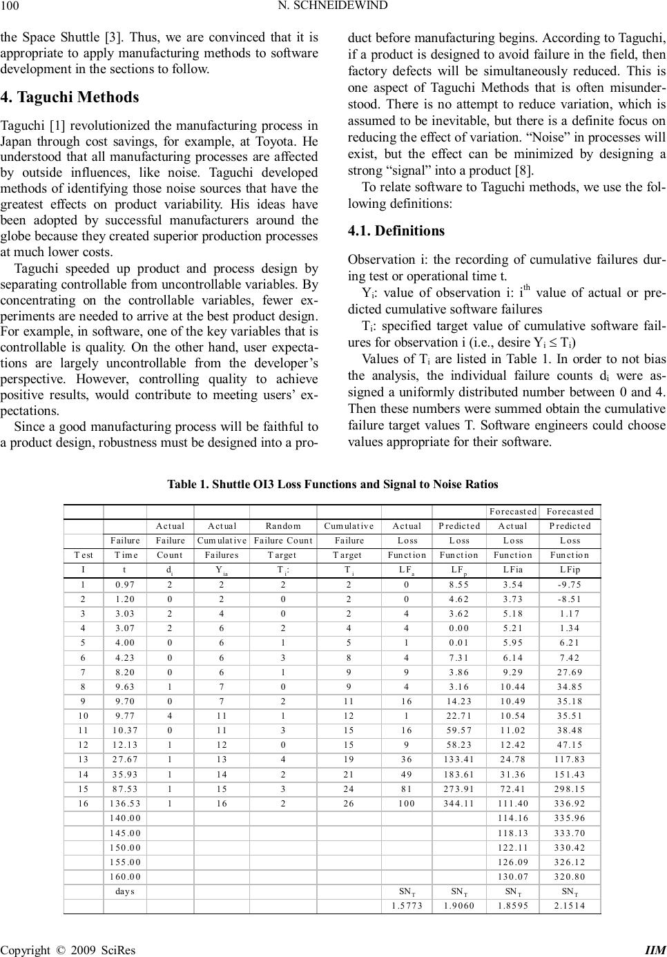

N. SCHNEIDEWIND 100
the Space Shuttle [3]. Thus, we are convinced that it is
appropriate to apply manufacturing methods to software
development in the sections to follow.
4. Taguchi Methods
Taguchi [1] revolutionized the manufacturing process in
Japan through cost savings, for example, at Toyota. He
understood that all manufacturing processes are affected
by outside influences, like noise. Taguchi developed
methods of identifying those noise sources that have the
greatest effects on product variability. His ideas have
been adopted by successful manufacturers around the
globe because they created superior production processes
at much lower costs.
Taguchi speeded up product and process design by
separating controllable from uncontrollable variables. By
concentrating on the controllable variables, fewer ex-
periments are needed to arrive at the best product design.
For example, in software, one of the key variables that is
controllable is quality. On the other hand, user expecta-
tions are largely uncontrollable from the developer’s
perspective. However, controlling quality to achieve
positive results, would contribute to meeting users’ ex-
pectations.
Since a good manufacturing process will be faithful to
a product design, robustness must be designed into a pro-
duct before manufacturing begins. According to Taguchi,
if a product is designed to avoid failure in the field, then
factory defects will be simultaneously reduced. This is
one aspect of Taguchi Methods that is often misunder-
stood. There is no attempt to reduce variation, which is
assumed to be inevitable, but there is a definite focus on
reducing the effect of variation. “Noise” in processes will
exist, but the effect can be minimized by designing a
strong “signal” into a product [8].
To relate software to Taguchi methods, we use the fol-
lowing definitions:
4.1. Definitions
Observation i: the recording of cumulative failures dur-
ing test or operational time t.
Yi: value of observation i: ith value of actual or pre-
dicted cumulative software failures
Ti: specified target value of cumulative software fail-
ures for observation i (i.e., desire Yi ≤ T i)
Values of Ti are listed in Table 1. In order to not bias
the analysis, the individual failure counts d
i
were as-
signed a uniformly distributed number between 0 and 4.
Then these numbers were summed obtain the cumulative
failure target values T. Software engineers could choose
values appropriate for their software.
Table 1. Shuttle OI3 Loss Functions and Signal to Noise Ratios
Forecasted Forecasted
Actual Actual Random Cumulative Actual Predicted Actual Predicted
Failure Failure Cumulative Failure Count Failure Loss Loss Loss Loss
Test Time Count FailuresTarget Target Function Function Function Function
I tdiYia Ti:T iLFaLFpLFia LFip
10.97 222208.55 3.54-9.75
21.20 020204.62 3.73-8.51
33.03 240243.62 5.18 1.17
43.07 262440.00 5.21 1.34
54.00 061510.01 5.95 6.21
64.23 063847.31 6.14 7.42
78.20 061993.86 9.29 27.69
89.63 170943.16 10.44 34.85
99.70 0721116 14.23 10.49 35.18
10 9.77 411112122.71 10.54 35.51
11 10.37 01131516 59.57 11.02 38.48
12 12.13 112015958.23 12.42 47.15
13 27.67 11341936 133.41 24.78 117.83
14 35.93 11422149 183.61 31.36 151.43
15 87.53 11532481 273.91 72.41 298.15
16 136.53 116226 100 344.11 111.40336.92
140.00 114.16335.96
145.00 118.13333.70
150.00 122.11330.42
155.00 126.09326.12
160.00 130.07320.80
days SNTSNTSN TSNT
1.5773 1.9060 1.85952.1514

N. SCHNEIDEWIND
101
LF: loss function (variability of difference between
actual cumulative failures and target values during test-
ing and operation)
SNT: signal to noise ratio (proportional to the mean of
the loss function)
n: number of observations (e.g., number of observa-
tions of Yi and Ti)
Taguchi devised an equation -- called the loss function
(LF) -- to quantify the decline of a customer's perceived
value of a product as its quality declines [9,10] in Equa-
tion (1). This equation is a squared error function that is
used in the analysis of errors resulting from deviations
from desired quality. LF tells managers how much prod-
uct quality they are losing because of variability in their
production process. He also computed his version of the
signal to noise ratio that essentially produces the mean of
the loss function [9,10] in Equation (2). Note that in most
applications, a high signal to noise ratio is desirable.
However, in the Taguchi method this is not the case be-
cause Equation (2) only measures signal, and no noise.
Thus, since Equation (2) represents the mean value of the
difference between observed and target values, a high
value of SNT is undesirable.
LF = (Yi – Ti)2, (1)
SNT =
2
1
10
()
10log()
n
ii
i
YT
n
=
−
∑ (2)
The development of the loss function and signal to
noise ratio, using the Shuttle failure data, involves the
following steps:
1) First, we note that cumulative failure data are ap-
propriate for comparing actual failure of a software re-
lease against the predicted values [11].
2) Thus, for release OI3 of the Shuttle flight software,
we used actual cumulative failure data Y
ia to compute
the actual loss function LFa in Equation (1).
3) Then we used this loss function to compute the ac-
tual signal to noise ratio SNT in Equation (2).
4) Then we used the predicted cumulative failure data
Yip to obtain the predicted loss function LFp and used
this loss function to compute the predicted signal to
noise ratio. The predicted cumulative failure counts were
obtained from another research project using the Schn-
eidewind Software Reliability Model (SSRM) [12]. Note
in Figure 1 that there is a good fit with the actual data
with R2 = .9359. Also note that the failure times are long
because the Shuttle flight software is subjected to con-
tinuous testing over many years of operation.
5) Next, the actual failure data Yia were fitted, as a fu-
nction of failure time t, with the regression Equation (3).
6) Then predicted failure data Y
ip were fitted, as a
function of failure time t, in the regression Equation (4),
which also has a good fit to the data in Figure 1 with R2
= .9701.
7) Finally, signal to noise ratios were computed using
Equation (2) for each of the four cases.
LFia=0.7956t+2.7771 (3)
LFip =-0.0204t2+5.3622t-14.912 (4)
The four loss functions -- two actual and two predicted
– are shown in Table 1 and Figure 1, along with the four
corresponding signal to noise ratios. Figure 1 and Equa-
tions (3) and (4) can be used by a software engineer to
forecast the loss function beyond the range of the actual
and predicted loss functions.
4.2. Results of Applying Taguchi Methods to
Shuttle Software
In Figure 1 and Table 1, we see that the loss functions
Figure 1. NASA space shuttle OI3: Loss function LF vs. failure time t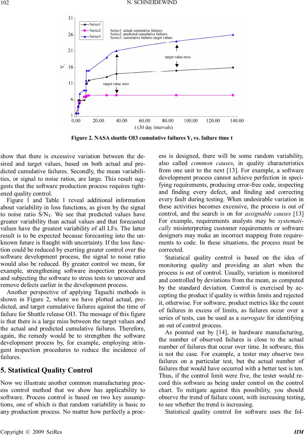

N. SCHNEIDEWIND 102
Figure 2. NASA shuttle OI3 cumulative failures Yi vs. failure time t
show that there is excessive variation between the de-
sired and target values, based on both actual and pre-
dicted cumulative failures. Secondly, the mean variabili-
ties, or signal to noise ratios, are large. This result sug-
gests that the software production process requires tight-
ened quality control.
Figure 1 and Table 1 reveal additional information
about variability in loss functions, as given by the signal
to noise ratio S/NT. We see that predicted values have
greater variability than actual values and that forecasted
values have the greatest variability of all LFs. The latter
result is to be expected because forecasting into the un-
known future is fraught with uncertainty. If the loss func-
tion could be reduced by exerting greater control over the
software development process, the signal to noise ratio
would also be reduced. By greater control we mean, for
example, strengthening software inspection procedures
and subjecting the software to stress tests to uncover and
remove defects earlier in the development process.
Another perspective of applying Taguchi methods is
shown in Figure 2, where we have plotted actual, pre-
dicted, and target cumulative failures against the time of
failure for Shuttle release OI3. The message of this figure
is that there is a large miss between the target values and
the actual and predicted cumulative failures. Therefore,
again, the remedy would be to strengthen the software
development process by, for example, employing strin-
gent inspection procedures to reduce the incidence of
failures.
5. Statistical Quality Control
Now we illustrate another common manufacturing proc-
ess control method that we show has applicability to
software. Process control is based on two key assump-
tions, one of which is that random variability is basic to
any production process. No matter how perfectly a proc-
ess is designed, there will be some random variability,
also called common causes, in quality characteristics
from one unit to the next [13]. For example, a software
development process cannot achieve perfection in speci-
fying requirements, producing error-free code, inspecting
and finding every defect, and finding and correcting
every fault during testing. When undesirable variation in
these activities becomes excessive, the process is out of
control, and the search is on for assignable causes [13]
For example, requirements analysts may be systemati-
cally misinterpreting customer requirements or software
designers may make an incorrect mapping from require-
ments to code. In these situations, the process must be
corrected.
Statistical quality control is based on the idea of
monitoring quality and providing an alert when the
process is out of control. Usually, variation is monitored
and controlled by deviations from the mean, as computed
by the standard deviation. Control is exercised by ac-
cepting the product if quality is within limits and rejected
it, otherwise. For software, product metrics like the count
of failures in excess of limits, as failures occur over a
series of tests, can be used as a surrogate for identifying
an out of control process.
As pointed out by [14], in hardware manufacturing,
the number of observed failures is close to the actual
number of failures that occur over time. In software, this
is not the case. For example, a tester may observe two
failures on a particular test, but the actual number of
failures that would have occurred with a better test is ten.
Thus, if the control limit were five, the tester would re-
cord this software as being under control on the control
chart. To mitigate against this possibility, you should
observe the trend of failure count, with increasing testing,
to see whether the trend is increasing.
Statistical quality control for software uses the fol-

N. SCHNEIDEWIND
103
lowing definitions and quality control relationships:
5.1. Definitions
n: Sample size
di: failure count for test i
i
d
: Mean value of d
i
Sample i: ith observation of di during test i
s: Sample standard deviation of di
di (min): minimum value of di
di: (max) maximum value of di
5.2. Quality Control Relationships
For the case where the standard deviation is used to
compute limits, Equations (5) and (6) are used.
Upper Control Limit (UCL):
i
d
+ Z s (5)
Lower Control Limit (LCL):
i
d
- Z s (6)
where Z is the number of standard deviations from the
mean, which can be 1, 2, or 3, depending on the degree
of control exercised (Z = 1: tight control, Z =3: loose
control).
5.3. Results of Applying Statistical Quality Con-
trol Methods to Shuttle Software
Since the Shuttle is a safety critical system, we chose Z =
1 to provide tight control. Figure 3 reveals, as the Ta-
guchi methods did, that there is an out of control situa-
tion when failure count become excessive -- in this case
at test # 10. In combining the results from Taguchi
methods and statistical quality control, corrective action,
like increased inspection, is necessary.
-
0.50
0.00
0.50
1.00
1.50
2.00
2.50
3.00
3.50
4.00
4.50
1
2
3
4
5
6
7 8
9
10
11
12 13 14 15 16
i
d
i
Series1
Series2
Series3
Series4
Series 1: d
i
Series 2: Mean d
i
Series 3: Mean d
i
+ 1 Standard Deviation
Series 4: Mean d
i
- 1 Standard Deviation
out of control
Figure 3. NASA space shuttle OI3: Failure count di vs. test i
Figure 4. NASA space shuttle OI3: Probability of di failures P (di) on n tests vs. di

N. SCHNEIDEWIND 104
4
3 2
1
0
6
5
4
3
2
1
0
Value
Expected
Observed
Figure 5. Test of poisson distribution of di number of failures during test i
6. Statistical Process Control Using Failure
Probability and Failure Counts [15]
Next we show other methods of statistical process con-
trol that focuses on the probability of failures and num-
ber of failures occurring in a sample on a test.
6.1. Probability of Failures during Tests
We use probability of failure P (di) of di failures during n
tests to control quality. This approach is based on the
binomial distribution with probability p
i
of failures on
test i [16]. In our example, using the Shuttle data, the
probability of failures P (di) is computed from the failure
counts di and pi in Equation (8). In order to compute P (di),
we first compute probability pi in Equation (7).
pi = di / n (7)
P (di) =n!
[][p[(1-p)]
d! (n-d)!
dn-d
]
ii
ii
ii
(8)
Applying Equation (8) to Figure 4, we note that there
would be considerable risk in deploying this software in
view of the high probability of failure for 2, 3, and 4
failures, given that 16 tests were used. An obvious rem-
edy for this problem would be to remove the faults caus-
ing the failures before the software is deployed.
6.2. Poisson Control Charts
The Poisson control chart is based on the assumption that
failure counts are distributed during tests according to a
Poisson distribution. As can be seen in Figure 5, the ob-
served failure counts di on the x axis are a good match
with the expected counts for a Poisson distribution.
Therefore, the Poisson distribution of failure counts,
given in Equation (9), is used. There is sometimes a con-
cern that the Poison distribution requires the assumption
of independence of failures. Actually, dependence is not
a frequent occurrence. For example, Musa [17] found
that in 15 projects there was little association among
failures.
pi = de
d!
_
d
_i
-d
i
(9)
Next, having estimated pi in Equation (9), estimate the
weighted mean number of failures across n samples, us-
ing Equation (10):
P
=
1
n
ii
i
dp
=
∑ (10)
Since the standard deviation s of the Poisson distribu-
tion is equal to square root of the mean, we have:
s =
_
P
(11)
Now, compute the lower control limit for the number
of failures using Equations (10) and (11) and producing
Equation (12):
LCL =
P
- 3 s (12)
It is necessary to compute the lower limit in order to
identify quality that may be too high, resulting in waste
of resources on software that does not require high qual-
ity.
Then, compute the upper control limit for the number
of failures, again using Equations (10) and (11) and pro-

N. SCHNEIDEWIND
105
ducing Equation (13):
UCL =
P
+ 3 s (13)
Figure 6 confirms the result obtained in Figure 3 in
that there is loss of control at test # 10 where four fail-
ures occur. The faults causing these failures must be un-
covered and removed.
7. Design of Experiments [18]
The last method in manufacturing process control we
consider is the design of experiments that employs a hy-
pothesis about the difference between desired (target) and
actual values of a product attribute, such as cumulative
failures, using software tests as the experiments. The idea
is to use samples (software tests) and statistical tests to
estimate whether there is a significant difference between
desired and actual values of a product attribute. If the
difference is significant, it may be attributed to process
factors, such as deficient quality control. We apply this
method to Shuttle software.
First determine whether the data are approximately
normally distributed as required for using the t test [16].
In Figure 7 it is shown that the cumulative failure data Yi
are approximately normally distributed by virtue of the
data (red) dots being close to the normal (blue) line.
Figure 6. NASA space shuttle OI3; process control using poisson distribution: Number of failures di vs. test number i
Figure 7. Normality test of cumulative number of failures yia

N. SCHNEIDEWIND 106
Table 2. Shuttle OI3 design of experiments
Ti Yia
2 2 s t
2 4 1.7531
4 6 t table
5 6 α 0.05
8 6 df 15
9 6 No statistically
9 7 Significant difference
11 7
12 11
15 11
19 13
21 14
24 15
26 16
11.5000 8.6250
i
T i Y
7.8825 4.5295
i
T
S i
Y
S
Second, state the null H0 and alternate H1 hypotheses:
H0: there is no statistically significant difference be-
tween Ti and Yi
H1: there is a statistically significant difference be-
tween Ti and Yi
Third, compute the means of the cumulative failures
and the target cumulative failures in Equations (14) and
(15), respectively, and the standard deviation of the sum
of the variance of Y
i
, s
Y
2
, and variance of T
i
, s
T
2
, in
Equation (16)
_1
n
i
i
i
Y
Y
n
=
=
∑
(14)
_1
n
i
i
i
T
T
n
=
=
∑
(15)
s =
22
ii
YT
ss
+ (16)
Fourth, based on the outcome of these computations,
the t statistic is computed in Equation (17).
t =
__
()
ii
YT
s
− (17)
Fifth, a comparison is made between the value com-
puted from Equation (17) and the value obtained from
the t statistic table. If (t < table value), accept H
0
and
conclude that the difference between the target and actual
cumulative failures is not statistically significant; other-
wise, accept H
1
and conclude there is a difference, and
attempt to assign the cause and correct the problem (e.g.,
inadequate software testing).
Based on Table 2, we accept H0 and conclude there is
not a statistically significant difference between cumula-
tive failures and the target values, based on the computed
t = 1.2650 < t table = 1.7531. Thus with an error of α
= .05 of rejecting H
0
, when in fact it is true, we have
confidence that quality based on cumulative failures
meets its goal.
8. Conclusions
We have presented some process methods from the field
of manufacturing with the objective that the methods will
prove useful to software engineers. While software de-
velopment has some unique characteristics, we can learn
from other disciplines, where the methods have been
applied extensively on an international scale as part of a
total quality management plan. Such a plan recognizes
that process and product are intimately related and that
the objective of software process improvement should be
to improve software product quality.
The loss function and signal to noise ratio inspired by
Taguchi methods proved to be valuable techniques for
identifying and reducing excessive variation in software

N. SCHNEIDEWIND
107
quality. In addition, statistical process control provided a
method for identifying the test when the incidence of
software failures was out of control. This allows the
software engineer to estimate the number of tests to
conduct in order to determine whether the software
product is under control. Finally, design of experiments
methodology allowed us to conduct hypothesis tests to
estimate whether software product metrics were achiev-
ing their goals.
REFERENCES
[1] J. G. Monks, “Operations management,” Second Edition,
McGraw-Hill, 1996.
[2] A. L. Jacob and S. K. Pillai, “Statistical process control to
improve coding and code review,” IEEE Software, Vol.
20, No. 3, pp. 50–55, May/June, 2003.
[3] T. Keller and N. F. Schneidewind, “A successful applica-
tion of software reliability engineering for the NASA
space shuttle, ” Software Reliability Engineering Case
Studies, International Symposium on Software Reliability
Engineering, Albuquerque, New Mexico, November 4,
pp. 71–82, 1997.
[4] J. Q. Ning, “Component-based software engineering
(CBSE), ” 5th International Symposium on Assessment of
Software Tools (SAST’97), p. 0034, 1997.
[5] A. Sloane and W. Waite, “Issues in automatic software
manufacturing in the presence of generators,” Australian
Software Engineering Conference, p. 134, 1998.
[6] Y. L. Yang, M. Li, and Y. Y. Huang, “The use of configu-
ration conception in software development, ” IEEE Pa-
cific-Asia Workshop on Computational Intelligence and
Industrial Application, Vol. 2, pp. 963–967, 2008.
[7] R. V. Binder, “Can a manufacturing quality model work
for software?” IEEE Software, Vol. 14, No. 5, pp. 101 –
102,105, September/October 1997.
[8] M. Eiklenborg, S. Ioannou, G. King II, and M. Vilcheck,
“Taguchi methods for achieving quality,” San Francisco
State University, School of Engineering. http://userwww.
sfsu.edu/~gtarakji/engr801/wordoc/taguchi.html.
[9] R. K. Roy, “Design of experiments using the taguchi
approach: 16 steps to product and process improvement,”
John Wiley & Sons, Inc., 2001.
[10] G. Taguchi, S. Chowdhury, and Y. Wu, “Taguchi’s qual-
ity engineering handbook,” John Wiley & Sons, Inc.,
2005.
[11] Handbook of Software Reliability Engineering, Edited by
Michael R. Lyu, Published by IEEE Computer Society
Press and McGraw-Hill Book Company, 1996.
[12] N. F. Schneidewind, “Reliability modeling for safety
critical software, ” IEEE Transactions on Reliability, Vol.
46, No. 1, pp. 88–98, March 1997.
[13] http://highered.mcgraw-hill.com/sites/dl/free/0072498919
/95884/sch98919_ch09.pdf.
[14] N. Eickelmann and A. Anant, “Statistical process control:
What you don’t measure can hurt you!” IEEE Software,
Vol. 20, No. 2, pp. 49–51, March/April, 2003.
[15] W. C. Turner, J. H. Mize, and J. W. Nazemetz, “Introduc-
tion to industrial and systems engineering,” Third Edition,
Prentice Hall, 1993.
[16] D. M. Levine, P. P. Ramsey, and R. K. Smidt, “Applied
statistics for engineers and scientists,” Prentice-Hall,
2001.
[17] J. D. Musa, A. Iannino, and K. Okumoto, “Software reli-
ability: Measurement, prediction, application,” McGraw-
Hill, 1987.
[18] N. F. Fenton and S. L. Pfleeger, “Software metrics: A
rigorous & practical approach,” Second Edition, PWS
Publishing Company, 1997.