Intelligent Information Management, 2009, 1, 81-88
doi:10.4236/iim.2009.12013 Published Online November 2009 (http://www.scirp.org/journal/iim)
A Quantity Model for Controlling and Measuring
Software Quality Based on the Expert
Decision-Making Algorithm
Che-Wei CHANG1, Der-Juinn HORNG2, Hung-Lung LIN2
1Department of Information Management, Yuanpei University, Hsin Chu, Taiwan, China
2Department of Business Administration, National Central University, Jhongli City, Taiwan, China
Abstract: Researchers have been active in the field of software engineering measurement over more than 30
years. The software quality product is becoming increasingly important in the computerized society. Target
setting in software quality function and usability deployment are essential since they are directly related to
development of high quality products with high customer satisfaction. Software quality can be measured as
the degree to which a particular software program complies with consumer demand regarding function and
characteristics. Target setting is usually subjective in practice, which is unscientific. Therefore, this study
proposes a quantity model for controlling and measuring software quality via the expert decision-making al-
gorithm-based method for constructing an evaluation method can provide software in relation to users and
purchasers, thus enabling administrators or decision makers to identify the most appropriate software quality.
Importantly, the proposed model can provide s users and purchasers a reference material, making it highly
applicable for academic and government purposes.
Keywords: software quality characteristics, software quality model, multiple criteria decision making
(MCDM), analytic hierarchy process (AHP)
1. Introduction
The numerous challenges involved in software develop-
ment include devising quality software, accurately con-
trolling overhead costs, complying with a progress
schedule, maintaining the software system, coping with
unstable software systems and satisfying consumer de-
mand with respect to software quality [1–3]. These chal-
lenges may incur a software development crisis if per-
formed inefficiently. Problems within the software sector
can be summed up as follows: 1) Inability to accurately
forecast or control software development costs, 2) sub-
standard quality, poor reliability and ambiguous requests
on how to enhance requests by management directives
regarding, 3) unnecessary risks while offering and main-
taining quality assurance, and 4) high personnel turnover
rate, leading to lack of continuity and increased inci-
dence of defects in software development [4].
Researchers have been active in the field of software
engineering measurement over more than 30 years. The
software quality product is becoming increasingly im-
portant in the computerized society. Developing software
quality is complex and difficult, and so a firm must
maintain the software quality to gain a competitive ad-
vantage. However, when software quality is being de-
veloped, developers must simultaneously consider de-
velopmental budget, the schedule, the ease of mainte-
nance of the system and the user’s requirements. Users’
requirements and the management of software firms to-
gether determine the implementation of software sys-
tems.
Target setting in software quality function and usabil-
ity deployment are essential since they are directly re-
lated to development of high quality products with high
customer satisfaction. Software quality can be measured
as the degree to which a particular software program
complies with consumer demand regarding function and
characteristics (degree of conformity to requirements).
However, target setting is usually subjective in practice,
which is unscientific [5,6]. Therefore, this study proposes
a quantity model for controlling and measuring software
quality via the expert decision-making algorithm-based
method for constructing an evaluation method can pro-
vide software in relation to users and purchasers, thus
enabling administrators or decision makers to identify
the most appropriate software quality. Importantly, the
proposed model can provide s users and purchasers a
reference material, making it highly applicable for aca-
demic and government purposes.

C. W. CHANG ET AL.
82
2. Model for the Software Quality
Conversely, capability assessment frameworks usually
assess the process that is followed on a project in prac-
tice in the context of a process reference model, defined
separately and independently of any particular method-
ology [7]. Software architecture is a key asset in any or-
ganization that builds complex software-intensive sys-
tems. Because of its central role as a project blueprint,
organizations should first analyze the architecture before
committing resources to a software development pro-
gram [8]. To resolve the above problems, multi-attribute
characteristics or factors of software quality must be
considered. Effective management strategies in a tech-
nology setting are thus essential for resolving crises in
software development. Technological aspects are soft-
ware technology adopted and design expertise of a soft-
ware developer [4].
Multiple criteria decision making (MCDM) is a
methodology that helps decision makers make preference
decisions (e.g. assessment, ranking, selection) regarding
a finite set of available alternatives (courses of action)
characterized by multiple, potentially conflicting attrib-
utes [9,10]. MCDM provides a formal framework for
modeling multi-attribute decision problems, particularly
problems whose nature demands systematic analysis,
including analysis of decision complexity, regularity,
significant consequences, and the need for accountability
[9]. Among those well-known methods, MCDM has only
relatively recently been employed to evaluate software
quality performance. MCDM-based decision-making is a
wide method for the measuring the software quality
[4,11–13]. Among those well-known evaluation methods,
MCDM has been employed relatively recently to evalu-
ate organizational performance and it uses a set of attrib-
utes to resolve decision-making issues. Currently, one of
the most popular existing evaluation techniques was
performed by adopting the analytic hierarchy process
(AHP), which was utilized by setting up hierarchical or
skeleton within which multi-attribute decision problems
can be structured [13–18].
2.1. Analytic Hierarchic Process (AHP)
Assume that we have n different and independent criteria
(C1, C2, …, Cn) and they have the weights (W1, W2, …,
Wn), respectively. The decision-maker does not know in
advance the values of Wi, i = 1, 2, …, n, but he is capable
of making pair-wise comparison between the different
criteria. Also, assume that the quantified judgments pro-
vided by the decision-maker on pairs of criteria (Ci, Cj)
are represented in an matrix as in the following: nn

12
11 121 1
221 222
12
n
n
n
ij
nnn nn
CC C
aa a C
Ca aa
Aa
Caa a













If for example the decision-maker compares C1 with
C2, he provides a numerical value judgment a12 which
should represent the importance intensity of C1 over C2.
The a12 value is supposed to be an approximation of the
relative importance of C1 to C2; i.e., .
This can be generalized and the following can be con-
cluded:
121 2
(/ )aWW
,

n
(1)
1) 121 2
(/) , 1,2,...,.aWWij


2) 1, 1, 2, ..., .
ii
ai n


3) If , 0, than 1/, 1, 2, ..., .
ij ji
aain




4) If is more important than , than
i
Cj
C12
a

.
12
)(/WW 1
This implies that matrix A should be a positive and re-
ciprocal matrix with 1’s in the main diagonal and hence
the decision-maker needs only to provide value judg-
ments in the upper triangle of the matrix. The values as-
signed to aij according to Saaty scale are usually in the
interval of 1 - 9 or their reciprocals. Table 1 presents
Saaty’s scale of preferences in the pair-wise comparison
process. It can be shown that the number of judgments (L)
needed in the upper triangle of the matrix are:
(1)/2,Lnn

 (2)
where n is the size of the matrix A:
Having recorded the numerical judgments aij in the
matrix A, the problem now is to recover the numerical
weights (W1, W2, …, Wn) of the criteria from this matrix.
In order to do so, consider the following equation:
11 121
21 222
12
n
n
nn nn
aa a
aa a
aaa












  
  

 

111 21
212 22
12
.
/ / /
/ / /
/ / /
n
n
nn n
WW WWWW
WW WWWW
WW WWWW
n



















(3)
Moreover, by multiplying both matrices in Equation (3)
on the right with the weights vector 12
where W is a column vector. The result of the multiplica-
tion of the matrix of pair-wise ratios with W is nW, hence
it follows:
(, , ..., ),
n
WWW W
.
A
WnW

 (4)
This is a system of homogenous linear equations. It
has a non-trivial solution if and only if the determinant of
A
nI

vanishes, that is, n is an eigenvalue of A. I is an
nn

identity matrix. Saaty’s method computes W as
the principal right eigenvector of the matrix A, that is,

C. W. CHANG ET AL.
83
Table 1. Saaty’s scale of preferences in the pair-wise comparison process
Numerical Verbal judgments of preferences between Ci and Cj
1 i is equally important to j
3 i is slightly more important than j
5 i is strongly more important than j
7 i is very strongly more important than j
9 i is extremely more important than j
2, 4, 6, 8 Intermediate values
Table 2. Average random index for corresponding matrix size
(n) 1 2 3 4 5 6 7 8 9 10 11 12 13 14 15
(R.I.) 0 0 0.58 0.90 1.12 1.24 1.32 1.41 1.45 1.49 1.51 1.48 1.56 1.57 1.59
max
A
WW

 (5)
where max

is the principal eigenvalue of the matrix A.
If matrix A is a positive reciprocal one then ,
max n


[19]. The judgments of the decision-maker are perfectly
consistent as long as
, , , 1, 2, ..., ,
ij jkik
aaai j kn (6)
which is equivalent to
(/ )(/ )(/ ),
ijjk ik
WW W WWW

(7)
The eigenvector method yields a natural measure of
consistency. Saaty defined the consistency index (C.I.) as
.. ()/(1).
max
CIn n

  (8)
For each size of matrix n; random matrices were gen-
erated and their mean C.I. value, called the random index
(R.I.), was computed and tabulated as shown in Table 2.
Accordingly, Saaty defined the consistency ratio as
.../ ..CRCIRI. (9)
The consistency ratio C.R. is a measure of how a given
matrix compares to a purely random matrix in terms of
their consistency indices. A value of the consistency ratio
is considered acceptable. Larger values of C.R.
require the decision-maker to revise his judgments.
.. 0.1CR 
3. Case Implementation
The city government of Hsinchu, in northern Taiwan,
intends to implement a system for monitoring public
spaces. Hence, the Hsinchu City Government is install-
ing digital video recorder systems (DVRs). in place of
traditional surveillance camera systems. The DVRs cir-
cumvents restrictions corrects the limitations of tradi-
tional surveillance camera systems, which include: a)
lapses in recording due to operator neglect or machine
error; b) difficulty in locating a desired time sequence
following completion of a recording; c) poor video qual-
ity and d) difficulty in maintaining and preserving tapes
due to a lack storage space and natural degradation of
film quality.
According to government procurement regulations,
regional governments must select at least five evaluators
to review more than three firms before evaluating the
best DVRs software quality. This study considers four
candidate DVRs software packages common in the sur-
veillance market manufactured by Firms A, B, C and D.
As Figure 1 shows, the ISO 9126-1 standard was de-
veloped in 2001 not only to identify major quality attrib-
utes of computer software, but also as a measure of six
major quality attributes. The proposed method adopts the
ISO 9126-1 model to evaluate the DVRs software quality.
The applicability of the proposed model is demonstrated
in a case study. This model for evaluating the DVRs
software quality comprises the following steps.
3.1. Step 1: Establish an Evaluation Model and
Define the Criteria
Evaluate the ideal model, as six evaluation criteria,
twenty-one sub-criteria and, finally, comparison with
four alternatives (Figure 1). The evaluation criteria and
sub-criteria used to evaluate the DVRs software quality
are defined as follows:
 Functionality (C1): The degree to which the soft-
ware satisfies stated requirements, including the four
sub-criteria of suitability, accuracy, interoperability and
security.
 Suitability: capability of software to provide an ap-
propriate set of functions for specified tasks and
user objectives.
 Maturity: capability of software to avert failure
caused by software defects.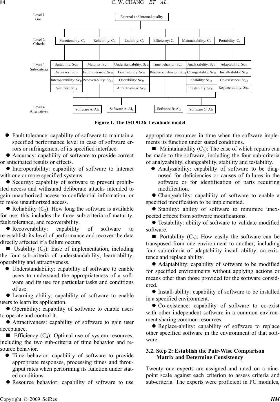

C. W. CHANG ET AL.
84
Level 1
Goal
Level 2
Criteria
Level 3
Sub-criteria
Level 4
Alternatives
Interoperability: Sc13
Suitability: Sc11
Accuracy: Sc12
Security: Sc14
Maturity: Sc21
Fault tolerance: Sc22
Recoverability: Sc23
Understandability: Sc31
Learn-ability: Sc32
Operability: Sc33
Time behavior: Sc41
Resource behavior: Sc42
Analyzability: Sc51
Changeability: Sc52
Stability: Sc53
Testability: Sc54
Adaptability: Sc61
Install-ability: Sc62
Co-existence: Sc63
Replace-ability: Sc64
External and internal quality
Functionality: C1 Reliability: C2 Usability: C3 Efficiency: C4 Maintainability: C5Portability: C6
Attractiveness: Sc34
Software A: Al1 Software B: Al2Software C: Al3
Software A: Al1
Figure 1. The ISO 9126-1 evaluate model
 Fault tolerance: capability of software to maintain a
specified performance level in case of software er-
rors or infringement of its specified interface.
 Accuracy: capability of software to provide correct
or anticipated results or effects.
 Interoperability: capability of software to interact
with one or more specified systems.
 Security: capability of software to prevent prohib-
ited access and withstand deliberate attacks intended to
gain unauthorized access to confidential information, or
to make unauthorized access.
 Reliability (C2): How long the software is available
for use; this includes the three sub-criteria of maturity,
fault tolerance, and recoverability.
 Recoverability: capability of software to
re-establish its level of performance and recover the data
directly affected if a failure occurs.
 Usability (C3): Ease of implementation, including
the four sub-criteria of understandability, learn-ability,
operability and attractiveness.
 Understandability: capability of software to enable
users to understand the appropriateness of a soft-
ware and its use for particular tasks and conditions
of use.
 Learning ability: capability of software to enable
users to learn its application.
 Operability: capability of software to enable users
to operate and control it.
 Attractiveness: capability of software to gain user
acceptance.
 Efficiency (C4): Optimal use of system resources,
including the two sub-criteria of time behavior and re-
source behavior.
 Time behavior: capability of software to provide
appropriate responses, processing times and throu-
ghput rates when performing its function under stat-
ed conditions.
 Resource behavior: capability of software to use
appropriate resources in time when the software imple-
ments its function under stated conditions.
 Maintainability (C5): The ease of which repairs can
be made to the software, including the four sub-criteria
of analyzability, changeability, stability and testability.
 Analyzability: capability of software to be diag-
nosed for deficiencies or causes of failures in the
software or for identification of parts requiring
modification.
 Changeability: capability of software to enable a
specified modification to be implemented.
 Stability: ability of software to minimize unex-
pected effects from software modifications.
 Testability: ability of software to validate modified
software.
 Portability (C6): How easily the software can be
transposed from one environment to another; including
four sub-criteria of adaptability install ability, co exis-
tence and replace ability.
 Adaptability: capability of software to be modified
for specified environments without applying actions or
means other than those provided for the software consid-
ered.
 Install-ability: capability of software to be installed
in a specified environment.
 Co-existence: capability of software to co-exist
with other independent software in a common environ-
ment sharing common resources.
 Replace-ability: capability of software to replace
other specified software in the environment of that soft-
ware.
3.2. Step 2: Establish the Pair-Wise Comparison
Matrix and Determine Consistency
Twenty one experts are assigned and rated on a nine-
point scale against each criterion to assess criteria and
sub-criteria. The experts were proficient in PC modules,

C. W. CHANG ET AL. 85
software modules and network communication modules.
The program adopted of the respondents’ data to cross-
compare all criteria and alternatives to determine the
weights and inconsistency ratios. The inconsistency ratio
is a measure of the percentage of time when decision
makers are inconsistent in making judgment. The “ac-
ceptable” inconsistency ratio was approximately 0.1 or
less, but “particular circumstance” may warrant the ac-
ceptance of a higher value. However, an inconsistency
ratio of 1 is unacceptable because the ratings are as good
as random judgments. Four of the twenty one experts had
inconsistency ratios above 0.15. This was too high and
their responses were discarded. Of the remaining seven-
teen, ten experts had low inconsistency ratios (<0.05),
and seven had ratios between 0.12 and 0.14. These seven
respondents were each given another chance to recheck
at their ratings and determine whether they would like to
modify their decisions, and eventually modified their
rating by making their own adjustments to the data.
Chang et al. proposal determining consistency procedure
as shows Figure 2.
After discarding ht responses of the four inconsistent
experts, the weights were then determined for a sample
group of seventeen individuals matching the above char-
acteristics with each respondent, making a pair-wise
comparison of the decision elements and assigning them
relative scores.
Pair-wise comparison matrix for each the
decision maker
Determine consistency
C.R.≦0.1
C.R. ＞ 0.1≦0.15
Discard decision matrix
Accept decision matrix
Given another chance to recheck at their ratings and
determine if they would like to change their decisions.
Determine eigenvectors (weights) for each
decision matrix
Using the geometric mean method
Figure 2. The procedure for determining consistency
Table 3. Aggregate pair-wise comparison matrix with eigenvectors
C1 C2 C3 C4 C5 C6 Eigenvectors
C1 1.000 0.812 0.474 0.321 0.722 1.182 0.108
C2 1.231 1.000 0.762 0.695 0.433 2.150 0.147
C3 2.110 1.313 1.000 0.913 1.167 1.909 0.207
C4 3.120 1.438 1.095 1.000 1.278 2.110 0.241
C5 1.385 2.310 0.857 0.782 1.000 1.636 0.198
C6 0.846 0.465 0.524 0.474 0.611 1.000 0.098
λ
max = 6.118, C.I. = 0.024, R I. = 1.24, C.R. = 0.019

C. W. CHANG ET AL.
86
Table 4. Summarizes eigenvectors (weights) results for levels 2 to 4
Weights for level 4
Criteria Weights
for level 2 Sub-Criteria Weights for level 3
Weights of the
overall
Al1 Al2 Al3 Al4
SC1 0.207 0.041 0.290 0.300 0.152 0.258
SC2 0.157 0.035 0.316 0.281 0.140 0.263
SC3 0.258 0.052 0.278 0.260 0.180 0.282
C1 0.108
SC4 0.378 0.060 0.296 0.309 0.126 0.269
SC5 0.236 0.067 0.266 0.465 0.105 0.164
SC6 0.354 0.057 0.240 0.348 0.190 0.222
C2 0.147
SC7 0.410 0.037 0.343 0.280 0.162 0.216
SC8 0.323 0.046 0.320 0.347 0.112 0.221
SC9 0.275 0.114 0.344 0.221 0.112 0.323
SC10 0.179 0.127 0.222 0.207 0.236 0.335
C3 0.207
SC11 0.223 0.058 0.217 0.140 0.372 0.271
SC12 0.475 0.035 0.213 0.180 0.338 0.269
C4 0.241 SC13 0.525 0.043 0.329 0.289 0.111 0.271
SC14 0.295 0.062 0.287 0.265 0.114 0.334
SC15 0.177 0.017 0.289 0.330 0.126 0.254
SC16 0.216 0.033 0.246 0.358 0.121 0.276
C5 0.198
SC17 0.312 0.024 0.330 0.306 0.100 0.264
SC18 0.172 0.024 0.314 0.387 0.138 0.162
SC19 0.336 0.041 0.406 0.246 0.103 0.245
SC20 0.244 0.035 0.207 0.526 0.112 0.155
C6 0.098
SC21 0.248 0.052 0.271 0.478 0.089 0.161
3.3. Step 3: Determine Eigenvectors
The relative scores provided by 11 experts were then
aggregated by the geometric mean method. Table 3 pre-
sents the aggregate pair-wise comparison matrix and the
consistency test for level 2. The eigenvectors (weighs)
for level 2 can be determined by the procedure described
in the previous section, and are as follows
1
2
3
4
5
6
0.108
0.147
0.207 .
0.241
0.198
0.098
C
C
C
C
C
C











(11)
The respective weights of the six evaluative criteria
are functionality (0.305), reliability (0.255), usability
(0.160), efficiency (0.092), maintainability (0.135) and
portability (0.053).
The eigenvectors (weighs) for level 3 can be deter-
mined by the procedure described in the previous section,
and are as follows
The twenty-one evaluative sub-criteria are weighted as
follows: suitability (0.207), accuracy (0.157), interopera-
bility (0.258), security (0.378), maturity (0.236), fault
tolerance (0.354), recoverability 0.410), understandabil-
ity (0.323), learn-ability (0.275), operability (0.179),
attractiveness (0.223), time behavior (0.475), resource
behavior (0.525), analyzability (0.295), changeability
(0.177), stability (0.216), testability (0.312), adaptability
(0.172), install-ability (0.336), co-existence (0.244) and
replace-ability (0.248). Table 4 summarizes eigenvectors
(weights) results for levels 2 to 4.
3.4. Step 4: Determine DVRs’ Software Quality
According to Table 4, the quality of the four DVRs’ soft-
ware programs are then determined by Equation (12).
Equation (12) indicates that the quality of the four DVRs’
software programs are as follows: DVR A = 0.300, DVR
B = 0.314, DVR C = 0.170 and DVR D= 0.277.

C. W. CHANG ET AL. 87
0.290 0.316 0.278 0.296 0.266 0.240 0.343 0.320 0.344 0.222 0.217 0.213 0.329 0.287 0.289 0.246 0.330 0.314 0.406 0.207 0.271
0.300 0.281 0.260 0.309 0.465 0.348 0.280 0.347 0.221 0.207 0.140 0.180 0.289 0.265 0.330 0.358 0.306 0.387 0.246 0.526 0.478
0.152 0.140 0.180 0.126 0.105 0.190 0.162 0.112 0.112 0.236 0.372 0.338 0.111 0.114 0.126 0.121 0.100 0.138 0.103 0.112 0.089
0.258 0.263 0.282 0.269 0.164 0.222 0.216 0.221 0.323 0.335 0.271 0.269 0.271 0.334 0.254 0.276 0.264 0.162 0.245 0.155 0.161
 
 
 
 
 
 
1
2
0.041
0.035
0.052
0.060
0.067
0.057
0.037
0.046
0.114
0.127
0.058
0.035
0.043
0.062
0.017
0.033
0.024
0.024
0.041
0.035
0.052
Al
Al



































3
4
(12)
0.300
0.314
0.170
0.277
Al
Al







The DVR B performed the best; end users must test
the stability of the system. The software products were
tested on an Intel Pentium 4 3.2GB, 1GB DDR400 RAM
PC and sixteen visual channels running Windows XP
Professional. Therefore, the mean CPU efficiency was
32%, and maximum efficiency was 43%. The mean
MEM loading was 10586 K, and the top loading was
11200 K. During a week of testing, the system never
crashed and never required automatic shutdown or restart.
Clearly, DVR B had the best software quality.
4. Conclusions
This study proposes a multi-criteria evaluation model
and algorithm capable of effectively evaluating software
quality from the perspective of users or purchasers, thus
enabling administrators or decision makers to identify
optimum software quality. Significantly, this study pro-
vides procurement personnel with an easily applied and
objective method of assessing the appropriateness of
software quality. Therefore, this study proposes a method
for identifying the best software quality from among
those offered by four firms, by considering multiple as-
sessment characteristics, improving upon the popular
MCDM approach to alternative prioritization. This study
presents an optimal operating model and algorithm for
monitoring software in relation to users and purchasers,
thus enabling administrators or decision makers to iden-
tify the most appropriate software quality. Based on the
measurement results in this study, software users and
developers can not only more thoroughly understand the
merits and limitations of software products, but also ul-
timately enhance its overall quality. Administrators or
decision makers adopt the measurement results of this
study to evaluate software quality.
REFERENCES
[1] H. Aras, S. Erdogmus, and E. Koc, “Multi-criteria selec-
tion for a wind observation station location using analytic

C. W. CHANG ET AL.
88
hierarchy process,” Renewable Energy, Vol. 29, 2004, pp.
1383–1392.
[2] V. Belton and T. J. Stewart, “Multiple criteria decision
analysis: An integrated approach,” Kluwer Academic
Publishers, Boston, 2002.
[3] G. P. Cesar, M. Tom, and H. S. Brian, “A Metamodel for
assessable software development methodologies,” Soft-
ware Quality Journal, Vol. 13, No. 2, pp. 195–214, 2005.
[4] C. W. Chang, C. R. Wu, and H. L. Lin, “Evaluating the
digital video recorder systems using analytic hierarchy
and analytic network processes,” Information Sciences,
Vol. 177, No. 16, pp. 3383–3396, 2007.
[5] C. W. Chang, C. R. Wu, and H. L. Lin, (2007b), “Inte-
grating fuzzy theory and hierarchy concepts to evaluate
software quality,” Software Quality Journal, Published
online, Vol. 11, No. 27, 2007.
[6] C. W. Chang, C. R. Wu, and H. L. Lin, “Group deci-
sion-making in a multiple criteria environment—A case
using the AHPGR model to assess digital video recorder
systems,” Journal of Testing and Evaluation, Vol. 36, No.
2, pp. 583–589, 2008.
[7] P. F. Hsu and B.-Y. Chen, “Developing and implementing
a selection model for bedding chain retail store franchisee
using Delphi and fuzzy AHP,” Quality and Quantity, Vol.
41, No. 2, pp. 275–290, 2007.
[8] ISO/IEC9126-1, “Software engineering-product quality-
Part1: Quality model,” 2001.
[9] G. Issac, C. Rajendran, and R. N. Anantharaman, “An
instrument for the measurement of customer perceptions
of quality management in the software industry: An em-
pirical study in India,” Software Quality Journal, Vol. 14,
No. 4, pp. 291–308, 2005.
[10] L. S. Jose and H. Ines, “An AHP-based methodology to
rank critical success factors of executive information
systems,” Computer Standards and Interfaces, Vol. 28, pp.
1–12, 2005.
[11] R. Kazman, L. Bass, M. Klein, T. Lattanze, and L. North-
rop, “A Basis for Analyzing Software Architecture
Analysis Methods,” Software Quality Journal, Vol. 13,
No. 4, pp. 329–355, 2005.
[12] T. M. Khoshgoftaar, A. Herzberg, and N. Seliya, “Re-
source oriented selection of rule-based classification
models: An empirical case study,” Software Quality
Journal, Vol. 14, No. 4, pp. 309–338, 2006.
[13] T. M. Khoshgoftaar, N. Seliya, and N. Sundaresh, “An
empirical study of predicting software faults with case-
based reasoning,” Software Quality Journal, Vol. 14, No.
2, pp. 85–111, 2006.
[14] L. Z. Lin, and T. H. Hsu, “The qualitative and quantita-
tive models for performance measurement systems: The
agile service development,” Quality & Quantity, Vol. 42,
No. 4, pp. 445–476, 2008.
[15] F. Liu, K. Noguchi, A. Dhungana, A. V. V. N. S. N.
Srirangam, and P. Inuganti, “A quantitative approach for
setting technical targets based on impact analysis in soft-
ware quality function deployment,” Software Quality
Journal, Vol. 14, No. 2, pp. 113–134, 2005.
[16] M. Mollaghasemi and J. Pet-Edwards, “Making multiple-
objective decisions,” Los Alamitos, IEEE Computer So-
ciety Press, CA, 1997.
[17] T. Rafla, P. N. Robillard, and M. C. Desmarais, (2007),
“A method to elicit architecturally sensitive usability re-
quirements: Its integration into a software development
process,” Software Quality Journal, Vol. 15, No. 2, pp.
117–133.
[18] T. L. Saaty, (1980), “The analytic hierarchy process,”
McGraw Hill, New York, NY.
[19] E. Tolgaa, M. L. Demircana, and C. Kahraman, “Operat-
ing system selection using fuzzy replacement analysis
and analytic hierarchy process,” International Journal of
Production Economics, Vol. 97, pp. 89–117, 2005.
[20] C. R. Wu, C. W. Chang, and H. L. Lin, “FAHP sensitivity
analysis for measurement nonprofit organizational per-
formance,” Quality & Quantity, Vol. 42, No. 3, pp.
283–302, 2008.