Intelligent Information Management, 2009, 1, 73-80
doi:10.4236/iim.2009.12012 Published Online November 2009 (http://www.scirp.org/journal/iim)
Solving Linear Systems via Composition of
their Clans
Dmitry A. ZAITSEV
Odessa National Telecommunication Academy, Kuznechnaya, Odessa, Ukraine
Abstract: The decomposition technique for linear system solution is proposed. This technique may be com-
bined with any known method of linear system solution. An essential acceleration of computations is ob-
tained. Methods of linear system solution depend on the set of numbers used. For integer and especially for
natural numbers all the known methods are hard enough. In this case the decomposition technique described
allows the exponential acceleration of computations.
Keywords: linear system, decomposition, clans, acceleration of computation
1. Introduction
The task of linear system solution is a classical task of
linear algebra [10]. There are a variety of known meth-
ods for linear system solution. It should be noted that the
choice of the method depends essentially on the set of
numbers used. More precise it depends on the algebraic
structure of the variables and coefficients. The solution
of system in fields and bodies, for example, in rational or
real numbers is the most studied. These algebraic struc-
tures allow the everywhere defined operation of division.
It is convenient to develop the simple and powerful
methods. Precise and approximate methods are distin-
guished. The most popular is Gauss method consisting in
consequent elimination of variables and obtaining the
triangular form of the matrix.
Ring algebraic structures such as integer numbers re-
quire special methods, as the division is not the every-
where-defined operation in a ring. There is known the
universal method using unimodular transformations of
matrix to obtain Smith normal form [10]. Result matrix
has diagonal form and allow the simple representation of
solutions. Unfortunately this method is exponential. Up
to present time were suggested a few more complex but
polynomial methods [3,7,8]. The most interesting is
founded on consequent solution of system in the classes’
fields of deductions modulo of prime numbers to con-
struct a target general integer solution of the system [3].
The development of such areas of computer science as
Petri net theory [6,13], logic programming [5], artificial
intellect [1] require to solve integer systems over the set
of nonnegative integer numbers. Notice that nonnegative
integer numbers form algebraic structure of monoid. In
monoid even the operation of subtraction is not every-
where defined. All the known methods of integer system
solution in nonnegative integer numbers are exponential
[2,4,9,12]. It makes significant difficulties in the applica-
tion of these methods to real-life systems analysis.
For example, if the complexity of method is about
2
q
,
where
q
is the dimension of the system, then to solve
the system with dimension 100 it is required about
30
10
operations. A computer with the performance
9
10
op-
erations per second will have executed this job in
21
10
seconds or in about
13
10
years.
Therefore, the task of the effective methods develop-
ment for linear system solution, especially in nonnega-
tive numbers, is enough significant. The goal of present
paper is to introduce the decomposition technique of
linear system solution. Application of this technique al-
lows an essential acceleration of computations. In the
case the exponential complexity of the source method of
system solution the acceleration is exponential too.
2. Basic Concepts
Let us consider a homogeneous linear system
0
Ax
⋅=
(1)
where
A
is the matrix of coefficients with dimension
of
mn
×
and
x
is the vector-column of variables with
dimension of
n
. So we have the system of
m
equa-
tions with
n
unknowns. We do not define now more
precisely the sets of variables and coefficients. We sup-
pose only that there is a method to solve a system (1) and
to represent the general solution in the form
xyG
=⋅
(2)
where matrix
G
is the matrix of basis solutions and
y

D. A. ZAITSEV 74
is the vector-row of independent variables. Each row of
matrix
G
is a basis solution. To generate a particular
solution of system the values of components of vector
y
may be chosen arbitrarily with respect to the set of
values of variables
x
. It should be noted that system (1)
has always at least the trivial zero solution. For the brev-
ity we shall name further homogeneous system an incon-
sistent in the case it has only the trivial solution.
Let us consider a nonhomogeneous system
Axb
⋅=
(3)
where
b
is the vector-column of free elements with
dimension of
m
. We suppose also that there is a method
to solve the system (3) and to represent the general solu-
tion in the form
xxyG
′
=+⋅
(4)
where
yG
⋅
is the general solution of corresponding
homogenous system (1) and
x
′
is the minimal particu-
lar solution of the nonhomogeneous system (3).
According to classical algebra [10], results represented
above are true for arbitrary fields and rings. Moreover,
according to [4], they are true also for monoid solutions
with a ring structure of matrix
A
and vector
b
. In this
case the set of minimal solutions
x
′
of nonhomogene-
ous system should be used.
3. Decomposition of System
Let us decompose the system (1) of homogeneous equa-
tions
0
Ax
⋅=
Above system may be considered as the predicate
12
()()()...()
m
LxLxLxLx
=∧∧∧ (5)
where
()
i
Lx
are the equations of the system:
()(0)
i
i
Lxax
=⋅=
and
i
a
is the i-th row of the matrix
A
. We imply that
i
a
is a nonzero vector so at least one component of
i
a
is nonzero. Moreover, we shall denote as
X
the set of
variables of system.
Let us consider the set of equations
{}
i
L
ℑ= of sys-
tem
L
. We shall introduce relations over the set
ℑ
.
Definition 3.1. Near relation: two equations ,
ij
LL
∈ℑ
are near and denoted as
ij
LL
o
if and only if k
xX
∃∈
:
,,
,0
ikjk
aa
≠
, ,,
()()
ikjk
signasigna=.
Lemma 3.1. Near relation is reflexive and symmetric.
Proof.
a) Reflexivity:
ii
LL
o
. As
i
a
is a nonzero vector
so there exists k
xX
∈
: ,
0
ik
a
≠
. Then it is trivial that
,,
()()
ikik
signasigna
=.
b) Symmetry:
ijji
LLLL
⇒
oo
. It is symmetric ac-
cording to symmetry of equality sign:
,,,,
()()()()
ikjkjkik
signasignasignasigna
=⇒=.
For each equation chosen we may construct the set of
near equations. It is useful to consider the transitive clo-
sure of near relation. We introduce the special notation
for this transitive closure.
Definition 3.2. Clan relation: two equations
,
ij
LL
∈ℑ
belong to the same clan and are denoted as
ij
LL
o
if and only if there exists a sequence (may be
empty) of equations 12
,,...,
k
lll
LLL
such that:
1... k
illj
LLLL
oooo
.
Theorem 3.1. Clan relation is the equivalence rela-
tion.
Proof. We have to prove that relation above is reflex-
ive, symmetric and transitive. We shall implement this in
a constructive way.
a) Reflexivity:
ii
LL
o
. As Definition 3.2 allows
the empty sequence and near relation is reflexive ac-
cording to Lemma 3.1, so clan relation is reflexive.
b) Symmetry:
ijji
LLLL
⇒
oo
. As
ij
LL
o
, so,
according to Definition 3.2, we may construct the se-
quence 12
,,...,
k
lll
LLL
such as 1... k
illj
LLLL
oooo
. Since
near relation is symmetry according to Lemma 3.1, we
may construct the reversed sequence
11
,,...,
kk
lll
LLL
−such
as 1 ...
k
jlli
LLLL
oooo
, then
ji
LL
o
.
c) Transitivity: ,
ijjlil
LLLLLL
⇒
ooo
. As
ij
LL
o
,
jl
LL
o
, so, according to Definition 3.2, we
may construct two sequences 12
,,...,
k
iii
LLL
σ=and
12
,,...,
r
lll
LLL
ς=such that 1...k
iiij
LLLL
oooo
and
1... r
jlll
LLLL
oooo
. Let us consider the concatenation
j
L
σς
. This sequence connects the elements
i
L
and
l
L
with the chain of elements satisfying the near relation.
Thus
il
LL
o
.
Corollary. Clan relation defines the partition of the set
ℑ
:
j
j
C
ℑ=
U
, ij CC
=∅
I
,
ij
≠
.
Definition 3.3. Clan: element of the partition
{,
}
ℑ
o
will be named a clan and denoted
j
C
. The variables
,
(){,:0}
jjj
iikki
XXCxxXLCa
==∈∃∈≠
will be
named variables of clan
j
C
.
Definition 3.4. Internal variable: variable
()
j
i
xXC
∈
is an internal variable of the clan
j
C
if and only if for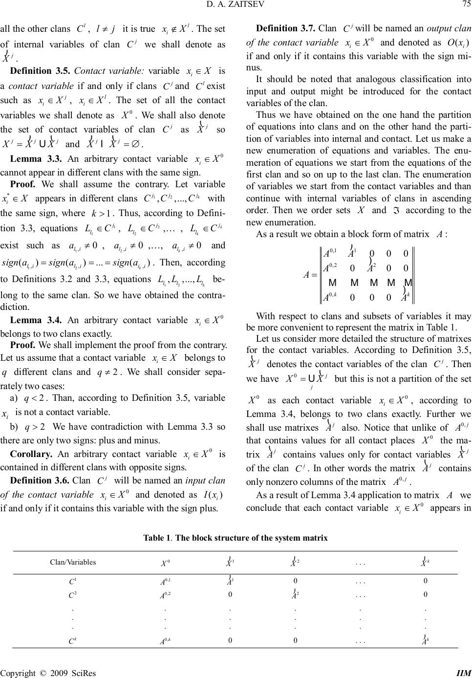

D. A. ZAITSEV
75
all the other clans
l
C
,
lj
≠
it is true
l
i
xX
∉. The set
of internal variables of clan
j
C
we shall denote as
j
X
)
.
Definition 3.5. Contact variable: variable i
xX
∈
is
a contact variable if and only if clans
j
C
and
l
C
exist
such as
j
i
xX
∈,
l
i
xX
∈. The set of all the contact
variables we shall denote as
0
X
. We shall also denote
the set of contact variables of clan
j
C
as
j
X
(
so
jjj
XXX
=
)(
U
and jj XX
=∅
)(
I
.
Lemma 3.3. An arbitrary contact variable
0
i
xX
∈
cannot appear in different clans with the same sign.
Proof. We shall assume the contrary. Let variable
*
i
xX
∈
appears in different clans 12
,,...,
k
j
jj
CCC
with
the same sign, where
1
k
>
. Thus, according to Defini-
tion 3.3, equations
1
1
j
l
LC
∈,
2
2
j
l
LC
∈,… ,
k
k
j
l
LC
∈
exist such as 1,
0
li
a
≠
, 2,
0
li
a
≠
,…, ,
0
k
li
a
≠
and
12
,,,
()()...()
k
liliii
signasignasigna=== . Then, according
to Definitions 3.2 and 3.3, equations 12
,,...,
k
lll
LLL
be-
long to the same clan. So we have obtained the contra-
diction.
Lemma 3.4. An arbitrary contact variable
0
i
xX
∈
belongs to two clans exactly.
Proof. We shall implement the proof from the contrary.
Let us assume that a contact variable i
xX
∈
belongs to
q
different clans and
2
q
≠
. We shall consider sepa-
rately two cases:
a)
2
q
<
. Than, according to Definition 3.5, variable
i
x is not a contact variable.
b)
2
q
>
We have contradiction with Lemma 3.3 so
there are only two signs: plus and minus.
Corollary. An arbitrary contact variable
0
i
xX
∈ is
contained in different clans with opposite signs.
Definition 3.6. Clan
j
C
will be named an input clan
of the contact variable
0
i
xX
∈ and denoted as
()
i
Ix
if and only if it contains this variable with the sign plus.
Definition 3.7. Clan
j
C
will be named an output clan
of the contact variable
0
i
xX
∈ and denoted as
()
i
Ox
if and only if it contains this variable with the sign mi-
nus.
It should be noted that analogous classification into
input and output might be introduced for the contact
variables of the clan.
Thus we have obtained on the one hand the partition
of equations into clans and on the other hand the parti-
tion of variables into internal and contact. Let us make a
new enumeration of equations and variables. The enu-
meration of equations we start from the equations of the
first clan and so on up to the last clan. The enumeration
of variables we start from the contact variables and than
continue with internal variables of clans in ascending
order. Then we order sets
X
and
ℑ
according to the
new enumeration.
As a result we obtain a block form of matrix
A
:
0,11
0,22
0,
000
000
000
kk
AA
AA
A
AA
=
)
)
MMMMM
)
With respect to clans and subsets of variables it may
be more convenient to represent the matrix in Table 1.
Let us consider more detailed the structure of matrixes
for the contact variables. According to Definition 3.5,
j
X
(
denotes the contact variables of the clan
j
C
. Then
we have 0
j
j
XX
=
(
U but this is not a partition of the set
0
X
as each contact variable
0
i
xX
∈, according to
Lemma 3.4, belongs to two clans exactly. Further we
shall use matrixes
j
A
(
also. Notice that unlike of
0,
j
A
that contains values for all contact places
0
X
the ma-
trix
j
A
(
contains values only for contact variables
j
X
(
of the clan
j
C
. In other words the matrix
j
A
(
contains
only nonzero columns of the matrix
0,
j
A
.
As a result of Lemma 3.4 application to matrix
A
we
conclude that each contact variable
0
i
xX
∈ appears in
Table 1. The block structure of the system matrix
Clan/Variables
0
X
1
X
)
2
X
)
. . .
k
X
)
1
C
0,1
A
1
A
)
0 . . . 0
2
C
0,2
A
0
2
A
)
. . . 0
.
.
.
.
.
.
.
.
.
.
.
.
.
.
.
.
.
.
k
C
0,
k
A
0 0 . . .
k
A
)

D. A. ZAITSEV 76
two of matrixes
0,
j
A
,
1,
jk
= exactly and besides, it
appears in one matrix with positive coefficients and in
another matrix with negative coefficients.
4. Solution of Decomposed System
At first we shall solve the system separately for each clan.
If we consider only variables of the clan we have the
system
0
jj
Ax
⋅=
(6)
where
,
j
jjjj
j
x
AAAx
x
==
(
()
)
.
System (6) will be denoted also as
()
j
C
Lx
. Notice
that values of variables
\
j
XX
may be chosen arbitrar-
ily. More detailed
()()
&
j
j
l
C
l
LC
LxLx
∈
=
Theorem 4.1. If system (1) has a nontrivial solution
then each system (6) has a nontrivial solution.
Proof. Let us consider the representation (5) of the
system (1). As, according to Theorem 3.1, clan relation
defines a partition of the set of equations, so representa-
tion (5) may be written in the form
12
()()()...()
k
CCC
LxLxLxLx
=∧∧∧ (7)
Thus, an arbitrary solution of (1) is the solution of
each system (6).
Corollary. If at least one of systems (6) is inconsistent
then the entire system (1) is inconsistent.
Let us the general solution of the system (6), accord-
ing to (2), has the form
jjj
xyG
=⋅
As each
j
i
xX
∈
)
is contained exactly in one system
(6), so for all the internal variables of clans we have
jjj
xyG
=⋅
)
)
Each contact variable, according to Lemma 3.4, be-
longs to two systems exactly. Thus, its values have to be
equal
or
jljjll
iiii
xxyGyG
=⋅=⋅
,
where
j
i
G
denotes the column of matrix
j
G
corre-
sponding to variable
i
x
.
Therefore, we obtain the system
0
,1,,
,,(),().
jjj
jjlljl
iiiii
xyGjk
yGyGxXCOxCIx
=⋅=


⋅=⋅∈==

(8)
Theorem 4.2. System (8) is equivalent to the system
(1).
Proof. As Expression (7) is the equivalent representa-
tion of the source system (1) and there is a partition of
the set of variables
X
into contact and internal, so above
reasoning proves the theorem.
Let us consider more detailed the equations of system
(8) for the contact variables. Equation
jjll
ii
yGyG
⋅=⋅
may be represented in a block form as
0
j
jl i
l
i
G
yy G
⋅=
−
We enumerate all the variables
j
y
in such a manner
to obtain the joint vector
12
...
k
yyyy
=
and assemble
j
i
G
,
l
i
G
into the joint matrix
F
. Thus,
we obtain the system
0
yF
⋅=
or
0
TT
Fy
⋅=
.(9)
System obtained has the form (1) so the general solu-
tion of system has the form (2):
yzR
=⋅
(10)
Let us compose the joint matrix
G
of systems’ (6)
solutions for all the clans in such a manner that
xyG
=⋅
(11)
This matrix has a block structure as follows
11
22
000
000
000
kk
SG
SG
G
SG
=
)
)
MMMMM
)
The structure of the first column of above block rep-
resentation that corresponds to contact variables is com-
plex enough. For each contact variable
0
i
xX
∈ we cre-
ate the column so that either block
j
S
or
l
S
contain
nonzero elements according to
j
G
(
or
l
G
(
where
()
j
i
COx
=,
()
l
i
CIx
=. Really, as a contact variable
belong to two clans, so its value may be calculated either
according to general solution of input clan or according
to general solution of output clan.
Let us substitute (10) into (11):
xzRG
=⋅⋅
Therefore
xzH
=⋅
,
HRG
=⋅
, (12)
Theorem 4.3. Expressions (12) represent the general

D. A. ZAITSEV
77
solution of homogeneous system (1).
Proof. As only equivalent transformations were used,
so above reasoning proves the theorem.
Let us implement analogous transformations for a
nonhomogeneous system (3). The general solution for
each clan, according to (4), has the form
jjjj
xxyG
′
=+⋅
Equations for contact variables may be represented as
follows
jjjlll
iiii
xyGxyG
′′
+⋅=+⋅
and further
jjll
iii
yGyGb
′
⋅−⋅=
,
lj
iii
bxx
′′′
=−
or in the joint matrix form
yFb
′
⋅=
or
TTT
Fyb
′
⋅=.
The general solution of above system, according to (4),
may be represented as
yyzR
′
=+⋅
.
Using the joint matrix
G
we may write
xxyG
′
=+⋅
or
(
)
xxyzRGxyGzRG
′′′′
=++⋅⋅=+⋅+⋅⋅
and finally
xyzH
′′
=+⋅
,
yxyG
′′′′
=+⋅
,
HRG
=⋅
. (13)
Theorem 4.4. Expressions (13) represent the general
solution of nonhomogeneous system (2).
Proof. As only equivalent transformations were used,
so above reasoning proves the theorem.
5. Description of Algorithm
Solution of linear homogeneous system of Equations (1)
with decomposition technique consists in:
Stage 1. Decompose system (1) into set of clans:
{}
j
C
.
Stage 2. Solve the system (6):
jjj
xyG
=⋅
for each
clan
j
C
. If at least one of systems (6) is inconsistent,
then the entire system (1) is inconsistent. Stop.
Stage 3. Construct and solve system (9) for contact
variables:
yzR
=⋅
. If this system is inconsistent, then
the entire system (1) is inconsistent. Stop.
Stage 4. Compose matrix
G
and calculate matrix
H
of basis solutions:
HRG
=⋅
. Stop.
It should be noted that Stages 2, 3 use a known method
of linear system solution. The choice of this method is
defined by the sets of numbers used. For example, this is
Gauss method for rational numbers, unimodular trans-
formations for integer numbers and Toudic method for
nonnegative integer solutions. Moreover, analogous
technique, according to Theorem 4.4, may be imple-
mented for nonhomogeneous system.
It has to describe more precisely now the decomposi-
tion algorithm used at Stage 1. Let us
q
is a maximum
dimension of matrix
A
:
max(,)
qmn
=. Clan relation
may be calculated in a standard way, as transitive closure
of near relation but this way is hard enough from the
computational point of view.
We propose the following algorithm of decomposition
(Figure 1) with a total complexity about
3
q
:
:1;
j
=
while
ℑ≠∅
do
:;
j
C
=∅
:,();
curCLL
=∈ℑ
:\;
L
ℑ=ℑ
do
:;
newC
=∅
for
L
′
in
curC
for
L
′′
in
ℑ
if
LL
′′′
o
then do
:\;
L
′′
ℑ=ℑ
:;
newCnewCL
′′
=
U
od;
:;
jj
CCcurC
=
U
:;
curCnewC
=
od until newC
=∅
:1;
jj
=+
od;
Figure 1. Algorithm of system decomposition

D. A. ZAITSEV 78
It creates clans
j
C
out of the source set of equations
ℑ
of the system. To create the transitive closure the
algorithm compares each equation of the set
curC
with
each equation of
ℑ
. Equations included into current
clan are extracted from the set
ℑ
. The usage of two
auxiliary subsets
curC
and
newC
allow the once
comparison of each pair of equations. As the calculation
of near relation is linear, so the total complexity of the
algorithm is about
3
q
.
Let us
()
Mq
is the time complexity of solution for
linear system of size
q
. We shall estimate the total
complexity of linear system solution with decomposition
technique. Let us the source system (1) is decomposed in
k
clans and
p
is the maximal number of either con-
tact or clans’ internal variables. Thus
(1)
qkp
≤+⋅
. The
following expression estimates the complexity of system
solution with decomposition technique:
33
()((1))()()((1))
VqkpkMpMpkp
≤+⋅+⋅+++⋅
.
Each of four addends of this expression estimates the complexity of the corresponding stage. In more simplified form
it is represented as
3333
()2(1)(1)()()
VqkpkMpkpkMp
≈⋅+⋅++⋅≈⋅+⋅ .
Let us estimate the acceleration of computations under
the decomposition technique usage. The target expres-
sion is
33
()
()
()
Mq
Accq
kpkMp
=⋅+⋅
It is enough clear that even for polynomial methods of
system solution with a degree higher than 3 we obtain
acceleration greater than one. Now we estimate the ac-
celeration for exponential methods with complexity
()2
q
Mq
=
such, for example, as Toudic method [9,12].
33
22
()2
22
qq
qp
pp
AccEq kpk
−
=≈=
⋅+⋅ .
The acceleration obtained is exponential. It is good
enough result.
6. Example
Let us solve the homogeneous system (1) of 9 equations
with 10 variables. The matrix of the system is as follows
1020011000
1000011000
0011020010
0011000010
0100001100
0100001102
0000100211
0000100011
0001100000
A
−−
−−
−−
−−
=−−
−−
−−
−−
−
Stage 1. Decomposition. Above system is decomposed
into two clans
1
1256
{,,,}
CLLLL
=, 2
34789
{,,,,}
CLLLLL
=.
It has the following subsets of clans’ variables
1
36810127
{,,,,,,}
Xxxxxxxx
=,
2
36810459
{,,,,,,}
Xxxxxxxx
=,
contact variables
012
36810
{,,,}
XXXxxxx
===
((
and internal variables
1
127
{,,}
Xxxx
=
)
, 2
459
{,,}
Xxxx
=
)
.
According to new enumeration of variables
(
)
36810127459
nx =
and new enumeration of equations
(
)
125634789
nL =
the matrix
A
has the form
2100101000
0100101000
0010011000
0012011000
1200000101
1000000101
0021000011
0001000011
0000000110
A
−−
−−
−−
−−
=
−−
−−
−−
−−
−
Stage 2. Solution of systems for clans. Application of
Toudic method gives us the following matrixes of basis
solutions for clans:
1
1100011
0011010
0000111
G=,

D. A. ZAITSEV
79
2
1111001
0000111
G=
with respect to vectors of free variables
1111
123
(,,)
yyyy
= and
222
12
(,)
yyy
= correspondingly.
Stage 3. Solution of system for contact variables. The
system for contact variables has the form:
12
11
12
11
12
21
12
21
0,
0,
0,
0.
yy
yy
yy
yy

−=

−=


−=


−=

It should be noted that equations correspond to contact
variables
36810
,,,
xxxx
and first and second equations
coincide as well as third and fourth. The general solution
of this system is
11010
00100
00001
R=
Stage 4. Composition of target solution. As it was
mentioned in section 4, matrix
G
may be composed in
different ways. Two variants of this matrix are repre-
sented as follows
1100011000
0011010000
0000111000
0000000001
0000000111
G= or
0000011000
0000010000
0000111000
1111000001
0000000111
G= .
And finally the result matrix of basis solutions of the
system (1) has the form
1111021001
0000111000
0000000111
HRG=⋅= .
The result obtained coincides with the basis solutions
calculated in usual manner with Toudic method.
7. Conclusions
Present paper introduced new technique of linear system
solution with decomposition into clans. It is efficient in
the combination with methods of system solution more
hard than a polynomial of third degree and in the case the
system may be decomposed in more than one clan.
As a result of this technique application to various
matrixes it may be concluded that a good opportunity to
decomposition have sparse matrixes. This is realistic
enough situation as large-scale real-life models contain
well-localized interconnections of elements.
It should be noted also the relationship of technique
proposed with the decomposition of Petri nets [11]. We
may construct the matrix of directions
D
for an arbi-
trary matrix
A
of linear system as
()
DsignA
=. Ma-
trix
D
may be considered further as incidence matrix
of Petri net.
The most significant acceleration of computations was
obtained for Diophantine (integer) systems especially
solving over the set of nonnegative numbers. There are
only exponential methods for solution of such systems.
In this case the acceleration of computation obtained is
exponential.
REFERENCES
[1] F. Baader and J. Ziekmann, “Unification theory,” Hand-
book of logic in artificial intelligence and logic pro-
gramming, Oxford: Univ. Press, pp. 1–85, 1994.
[2] E. Contejan and F. Ajili, “Avoiding slack variables in solv-
ing linear Diophantine equations and inequations,” Theo-
retical Computer Science, Vol. 173, pp. 183–208, 1997.
[3] M. A. Frumkin, “Algorithm of system of linear equations
solution in integer numbers,” Research on Discrete Opti-
misation, Moskow, Nauka, pp. 97–127, 1976.
[4] S. L. Kryviy, “Methods of solution and criteria of com-
patibility of systems of linear Diophantine equations over
the set of natural numbers,” Cybernetics and Systems
Analysis, Vol. 4, pp. 12–36, 1999.
[5] J. Lloyd, “Foundation of logic programming,” Berlin,
Springer-Verlag, 1987.
[6] T. Murata, “Petri nets: Properties, analysis and applica-
tions,” Proceedings of IEEE, Vol. 77, No. 4, pp. 541–580
1989.
[7] L. Pottier, “Minimal solutions of linear diophantine sys-
tems: bounds and algorithms,” Proceedings of the Fourth
Intern. Conference on Rewriting Technique and Applica-
tion, Como, Italy, pp. 162–173, 1991.
[8] J. F. Romeuf, “A polynomial algorithm for solving sys-
tems of two linear Diophantine equations,” Theoretical
Computer Science, Vol. 74, No. 3, pp. 329–340, 1990.
[9] J. M. Toudic, “Linear algebra algorithms for the structural
analysis of petri nets,” Rev. Tech. Thomson CSF, Vol. 14,
No. 1, pp. 136–156, 1982.
[10] B. L. Van Der Warden, Algebra, Berlin, Heidelberg,

D. A. ZAITSEV 80
Springer-Verlag, 1971.
[11] D. A. Zaitsev, “Subnets with input and output places,”
Petri Net Newsletter, Vol. 64, pp. 3–6, 2003.
[12] D. A. Zaitsev, “Formal grounding of toudic mmethod,”
Proceedings of the 10th Workshop “Algorithms and Tools
for Petri Nets”, Eichstaett, Germany, pp. 184–190, Sep-
tember 26-27, 2003.
[13] D. A. Zaitsev and A. I. Sleptsov, “State equations and equi-
valent transformations of timed petri nets,” Cybernetics
and System Analysis, Vol. 33, No. 5, pp. 659– 672, 1997.