American Journal of Oper ations Research, 2011, 1, 229-235
doi:10.4236/ajor.2011.14026 Published Online December 2011 (http://www.SciRP.org/journal/ajor)
229
An Objective Penalty Functions Algorithm for
Multiobjective Optimization Problem
Zhiqing Meng, Rui Shen, Min Jiang
College of Business and Administration, Zhejiang University of Technology, Hangzhou, China
Received October 24, 2011; revised November 20, 2011; accepted December 7, 2011
Abstract
By using the penalty function method with objective parameters, the paper presents an interactive algorithm
to solve the inequality constrained multi-objective programming (MP). The MP is transformed into a single
objective optimal problem (SOOP) with inequality constrains; and it is proved that, under some conditions,
an optimal solution to SOOP is a Pareto efficient solution to MP. Then, an interactive algorithm of MP is
designed accordingly. Numerical examples show that the algorithm can find a satisfactory solution to MP
with objective weight value adjusted by decision maker.
Keywords: Multiobjective Optimization Problem, Objective Penalty Function, Pareto Efficient Solution,
Interactive Algorithm
1. Introduction
The interactive algorithm is very efficient in solving
multi-objective optimization problems of many fields,
while the penalty function is a very important method in
solving optimization problems with constraints. Hence,
based on objective penalty function, we propose an in-
teractive algorithm which provides a versatile tool in
finding solutions to multi-objective optimization prob-
lems with constraints. In solving multi-objective optimi-
zation problems, the interactive algorithm provides a
way to adjust objective weight value between the deci-
sion maker and computer, so that solution space is read-
ily understood, which also makes it easier in use and
more convenient in operation.
In this paper the following inequality constrained
multi-objective programming is considered:
  

12
min,, ,
s.t. ,0,1,2,,,
q
i

f
xfxfxfx
xXgx im




(MP)
where 1
:n
j
f
RR, 1 :n
i
g
RR

1, 2,,iI 
for
, and X is a sub-
set of .

1, 2,, q
n
R
jJ

m
It is good to find out a satisfactory solution to (MP)
such that all objective values are optimal, but this is ob-
viously difficult in general. Hence, lots of efforts have
been devoted to this area to find an efficient method, and
up until now many algorithms are presented [1-11].
In 1971, Benayoun et al. firstly presented an interac-
tive algorithm STEM for linear multiobjective program-
ming [1]. Its idea is the first in finding out a solution of
an ideal value to every objective, obtaining better solu-
tion by improving unsatisfactory objectives value, and
keeping within concession value of satisfactory objec-
tives. With man-machine conversation, interactive algo-
rithms provide a method to solve MP. There are many
interactive approaches, as it is not possible for a decision
maker to know all the objective values of MP. Then
through interactive algorithms, he may gradually learn
objective value changes and thus in the interactive pro-
cedure may determine his preferences to objectives. As
to the dissatisfactory objectives, he may get satisfactory
solution by modifying some parameters he gives, e.g. the
ideal objective values and the weights of objectives.
For example, Geoffrion, Dyer and Feinberg (1972)
gave an interactive approach to multi-criterion optimiza-
tion, where they defined a non-explicitly criterion func-
tions to show the DM’s overall preference [2]. Zionts
and Wallenius (1976) also presented a man-machine in-
teractive mathematical programming method, where the
overall utility function is assumed to be implicitly a lin-
ear function and more generally a concave function of
the objective functions [3]. Furthermore, Rosinger (1981)
studied the algorithm which is a modification of the
steepest ascent method, giving at each iteration a signifi-

Z. Q. MENG ET AL.
230
cant freedom and ease for the decision-maker’s self-ex-
pression, and requiring a minimal information on his
local estimate of the steepest-ascent direction [4]. Zionts
and Wallenius (1983) developed a method for interactive
multiple objective linear programming by assuming an
unknown pseudo concave utility function satisfying cer-
tain general properties [5]. Sadagopan and Ravinderan
(1986) developed several interactive procedures for
solving multiple criteria nonlinear programming prob-
lems based on the generalized reduced gradient method
for solving single objective nonlinear programming prob-
lems [6]. Siegfried (1990) presented an interactive algo-
rithm for nonlinear vector optimization problems, after
solving only two optimization problems [7]. Kassem
(1995) dealt with an interactive stability of multiobjec-
tive nonlinear programming problems with fuzzy pa-
rameters in the constraints [8]. Aghezzaf and Ouaderh-
man (2001) proposed an interactive interior point method
for finding the best compromise solution to a multiple
objective linear programming problem [9]. Abo-Sinna
and Abou-El-Enien (2006) extended the technique of
order preference by similarity ideal solution (TOPSIS)
for solving large scale multiple objective programming
problems involving fuzzy parameters [10]. Luque, Ruiz
and Steuer pointed out that many interactive algorithms
have two main features: 1) they help a decision maker
(DM) learn about a problem while solving it, and 2) they
put to work iteratively any new insights gained during
the solution process to help the DM navigate to a final
solution [11].
It is difficult to define an appropriate utility function
for MP in the interactive algorithms. By using objective
penalty functions as utility functions for MP, the paper
obtains a satisfactory solution, when the decision maker
is allowed, in the interactive algorithm, to choose another
weight of objectives for some dissatisfactory objectives
time and again. So our interactive algorithm has two ad-
vantages: 1) it is able to find out an efficient solution to
each new MP with better convergence, 2) it can control
the change of objectives such that a more satisfactory
solution is obtained. What needs to focus on for the deci-
sion maker is the objective changes. Numerical examples
show that the proposed interactive algorithm has faster
convergence effect in Section 3.
The remainder of this paper is organized as follows. In
Section 2, we provide results of the penalty problem of
MP with penalty parameters. In Section 3, we present an
interactive algorithm to solve the MP. Numerical exam-
ples show that the proposed algorithm has good conver-
gence and can control objective changes by changing
objective weights.
2. An Objective Penalty Function
In this section, an objective penalty function of (MP) is
introduced.
For (MP), let

 
max, 0
ii
gx gx


for iI

and
define a function as follows:
11
:QR R

2
, 0t
 
maxQt 
t
. Then Q is increasing and dif-
ferentiable at any 1
R

.
A feasible set of (MP) is denoted as



00, i
X
xXgx iI

. 0
x
X is called a Pareto
efficient solution if there is no 0
x
X such that




f
xfx and


f
xfx.
Let an objective weight value
be a given positive vector, and

12 , 0
T
q
 
1
,, 
M
R be objective
parameters of






,
q12
,,
f
xfxfx. Then define

 
0jj
jJ
f
xQfx 

M

.
Theorem 2.1 If
x
is an optimal solution to the fol-
lowing problem:


0
min s.t. 0
f
xxX
, (P
λ)
and for all jJ

,

j
M
fx, then
x
is a Pareto
efficient solution to (MP).
Proof. Suppose that
x
is not a Pareto efficient solu-
tion to (MP), then there is an 0
x
X
 such that




f
xfx
 and


f
xfx
. It follows from the
assumption that




f
xMfxM


, , jJ
and there is at least such a that
jJ




f
xMfxM


. Hence, we have




00
f
xfx
, which results in a contradiction.
From Theorem 2.1, we learn that a Pareto efficient
solution to (MP) can be found out by solving the single
objective problem (Pλ). Furthermore, the problem (Pλ)
can be transformed into an unconstrained optimization
by using nonlinear penalty function, which is defined as:






  
2
0
2
,,
.
i
iI
jj i
jJ iI
FxMf xMgx
Qf xMMgx










where 0M

. Consider the following nonlinear penalty
optimization problem:


0
min,, s.t.
F
xM xX  . P
λ(M)
Theorem 2.2 Suppose that M is constant, *
M
x
is an
optimal solution to Pλ(M), and for all ,
jJ


*
jM
M
fx. If *
M
x
is a feasible solution to (MP), then
*
M
x
is a Pareto efficient solution to (MP).
Proof. Let *
x
be an optimal solution to Pλ(M). From
the given conditions, we have

231 Z. Q. MENG ET AL.
 


** *
0
,, ,,
MM
*
0
f
xFxMFxMfx  
.
Since *
M
x
is a feasible solution to (MP) and *
x
is
an optimal solution to Pλ(M), 00
M
 
*

*
f
xfx. So,
*
M
x
is an optimal solution to Pλ(M). From Theorem 2.1,
*
M
x
is a Pareto efficient solution to (MP).
Theorem 2.1 and Theorem 2.2 give a good way to
solve (MP). The objective parameter M required in
Theorem 2.2 may exist, as shown in the following exam-
ple.
Example 2.1 Consider the MP problem:


22
121 2
12
min ,,
s.t. 0,0.
f
xxx x
xx


(P2.1)
It is clear that is a Pareto efficient
solution to (P2.1) and the objective value is (0, 0). Let’s
take M < 0, λ1 > 0 and λ2 > 0. Define the penalty func-
tion:


**
12
,0, xx 

0

2

 
 
2
2
112 2
12
,,max,0 max,0
max0,max0,.
Fx Mx Mx M
xx
  

It is clear that (x1, x2) = (0, 0) is an optimal solution to
Pλ(M) [with M < 0].
It is proved in [13] that the stability of constrained
penalty function can ensure exactness. So in this paper
we define the stability of objective penalty function to
ensure equivalence between Pλ(M) and (Pλ).
Let a perturbed problem of (Pλ) defined as


0
min
s.t. ,,1,2,,
ii
fx
x
Xg xsim P
λ(s)
where

12
,, ,
M
s
ss s.
Definition 2.1 For n
s
R, let x* be an optimal solu-
tion to (Pλ) and *
s
x
be an optimal solution to Pλ(s). If
 
**2
00 s
f
xfxMs ,
where
1
m
i
i
s
s

,

12
,, ,
M

s
ss s, then problem (Pλ)
is called stable for M.
Theorem 2.3 Let x* be an optimal solution to (Pλ).
Then, problem (Pλ) is stable for M if and only if x* is an
optimal solution to Pλ(M).
Proof. First, if problem (P
λ) is stable for M, it is
hereby proved that x* is an optimal solution to Pλ(M).
Assume that x* is not an optimal solution to Pλ(M), then,
there is some x′ such that


**
0
,, ,,

F
xMFx M fx 

.
That is
 

*
00 0 i
iI
fxfxM gxfx


   
.
If x′ is a feasible solution to (Pλ), we will get a contra-
diction. Since x* be an optimal solution to (Pλ), we have



*
00
f
xfx


such that





*
00 0
fx fxfx


 , then x* is not an
optimal solution to (Pλ). Hence, we have that x′ is not any
feasible solution to (Pλ) and . Let 0
i
iI
g







max,0
ii
sgx

 for . Let 1, 2,,im*
s
x
be an
optimal solution to Pλ(s′). So, it is clear to have




*
00 s
f
xfx

. We have


 


2
00
*
0
,,
si i
iI iI
*2
f
xMsfxMgx
FxMf x 








and




**2
0s
f
xfxMs

.
Hence, the problem (Pλ) is not stable for M.
Next, let’s prove that the problem (Pλ) is stable for M,
under the condition that if x* is an optimal solution to
Pλ(M). Let x*
s be an optimal solution to (Pλ(s)). Since x*
is an optimal solution to Pλ(M), we have




**2
0
,,

*
s
is
iI
F
xMfxMgx 



.
That is




**2
00
s
i
iI
f
xfxMs


.
We have that problem (Pλ) is stable for M.
Example 2.2 Consider the problem (P2.1) and its
(P2.1)(s):



22
121 2
112 2
min ,,
s.t. ,.
f
xxx x
x
sx s

 
(P2.1)(s)


*
1
max 0,
s
x
s

, max{0, –s2} is a Pareto efficient
solution to (P2.1)(s). Let’s take M < 0. Define the penalty
function:



 
22
22
112 2
12
,,max ,0max ,0
max0,max0,.
Fx Mx Mx M
xx
  


We have that stable condition holds as follows:

 

 


2
2
**
00 1211
2
22
2
12
max 0,
max0,
max0,max{0,}.
s
fx fxsM
sM
Ms s


 


Based on Theorem 2.2 and Theorem 2.3, we develop
an algorithm to compute (MP). It solves the problem
Pλ(M) sequentially and we name it Objective Penalty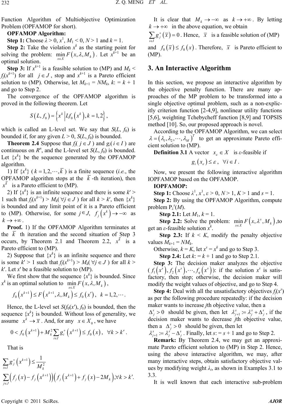

Z. Q. MENG ET AL.
232
Function Algorithm of Multiobjective Optimization
Problem (OPFAMOP for short).
OPFAMOP Algorithm:
Step 1: Choose λ > 0, x1, M1 < 0, N > 1 and k = 1.
Step 2: Take the violation xk as the starting point for
solving the problem:


min, ,k
xX
F
xM 
. Let xk+1 be an
optimal solution.
Step 3: If xk+1 is a feasible solution to (MP) and Mk <
fj(xk+1) for all , stop and xk+1 is a Pareto efficient
solution to (MP). Otherwise, let Mk+1 = NMk, k: = k + 1
and go to Step 2.
jJ
The convergence of the OPFAMOP algorithm is
proved in the following theorem. Let





00
,,
kk
SLfx Lfxk1,2,
which is called an L-level set. We say that S(L, f0) is
bounded if, for any given L > 0, S(L, f0) is bounded.
Theorem 2.4 Suppose that fj() and gi(ijJI

) are
continuous on Rn, and the L-level set S(L, f0) is bounded.
Let {xk} be the sequence generated by the OPFAMOP
algorithm.
1) If {xk} (1, 2,,kk ) is a finite sequence (i.e., the
OPFAMOP algorithm stops at the k-th iteration), then
k
x
is a Pareto efficient to (MP).
2) If {xk} is an infinite sequence and there is some k′ >
1 such that fj(xk+1) > Mk() for all k > k′, then {xk}
is bounded and any limit point of it is a Pareto efficient
to (MP). Otherwise, for some jJ, as
.
jJ

k
j
fx
k
Proof. 1) If the OPFAMOP Algorithm terminates at
the k th iteration and the second situation of Step 3
occurs, by Theorem 2.1 and Theorem 2.2, k
x
is a
Pareto efficient to (MP).
2) Suppose that {xk} is an infinite sequence and there
is some k′ > 1 such that fj(xk+1) > Mk() for all k >
k′. Let x' be a feasible solution to (MP).
jJ
We first show that the sequence {xk} is bounded. Since
xk is an optimal solution to

min, ,k
xX
F
xM 


,
 

11
00
,,
kk
k
f
xFxMfx 
 

, . 1, 2,k
Hence, the L-level set S(f0(x′), f0) is bounded, then the
sequence {xk} is bounded. Without loss of generality, we
assume k
x
x. And, for any 0
x
X, we have
 

12 1
00
0kk
ki
iI
f
xMgx f


 
x, kk

 .
That is







1
2
11
1
2,
k
j
iI k
kk
jjjj k
jJ
gx M
It is clear that k as . By letting
in the above equation, we obtain
M k
k



0
j
iI
gx
.
f
xfxfxfx Mkk












. Hence,

x
is a feasible solution of (MP)
and




00
f
xfx. Therefore,
x
is Pareto efficient to
(MP).
3. An Interactive Algorithm
In this section, we propose an interactive algorithm by
the objective penalty function. There are many ap-
proaches of the MP problem to be transformed into a
single objective optimal problem, such as a non-explic-
itly criterion function [2-4,9], nonlinear utility functions
[5,6], weighting Tchebycheff function [8,9] and TOPSIS
method [10]. So, our proposed approach is novel.
According to the OPFAMOP Algorithm, we can select
to get an approximate Pareto effi-
cient solution to (MP).

12
,,, T
M
  

Definition 3.1 A vector
x
X

 is ε-feasible if


i
gx



, . iI
Now, we present the following interactive algorithm
IOPFAMOP based on the OPFAMOP.
IOPFAMOP:
Step 1: Choose λ1, x1, ε > 0, N > 1, K > 1 and s = 1.
Step 2: By using the OPFAMOP Algorithm, compute
problem Pλ
s(M).
Step 2.1: Let M1, k = 1.
Step 2.2: Solve the problem:

min, ,
s
k
xX
F
xM 
,to
get an ε-feasible solution xk.
Step 2.3: If k < K, modify the penalty objective
values Mk+1 = NMk.
Otherwise, k = K, let xs = xk and go to Step 3.
Step 2.4: Let k: = k + 1 and go to Step 2.1.
Step 3: The decision maker analyzes the objective
(






12
,,,
s
s
q
s
f
xfx fx): if the solution xs is satis-
factory, then stop; otherwise, the decision maker will
modify the weight values of objective, and go to Step 4.
Step 4: Deal with all the unsatisfactory objectives fj(xs)
as per the following procedure repeatedly: if the decision
maker wants to increase jth objective value, then a
0
s
j

 should be given, then let 1:
s
ss
j
j

 j
, if the
decision maker wants to decrease jth objective value,
then a 0
s
j

 should be given, then let
1:
s
ss
j
jj



 . Finally, let s: = s + 1 and go to Step 2.
Remark: By Theorem 2.4, we may get an approxi-
mate Pareto efficient solution to (MP) in Step 2. Hence,
using the above interactive algorithm, we may, after
many interactive steps, obtain satisfactory objective val-
ues by modifying weight λi, as shown in Examples 3.1 to
3.3.
It is well known that each interactive sub-problem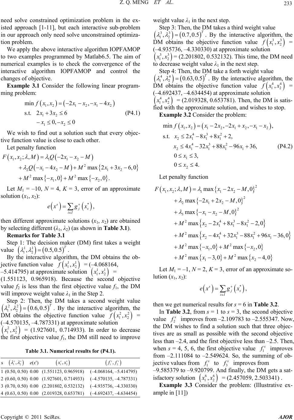

Z. Q. MENG ET AL. 233

need solve constrained optimization problem in the ex-
isted approach [1-11], but each interactive sub-problem
in our approach only need solve unconstrained optimiza-
tion problem.
We apply the above interactive algorithm IOPFAMOP
to two examples programmed by Matlab6.5. The aim of
numerical examples is to check the convergence of the
interactive algorithm IOPFAMOP and control the
changes of objective.
Example 3.1 Consider the following linear program-
ming problem:

121 212
12
12
min ,2,4
s.t. 236
0,0
f
xxx xxx
xx
xx



(P4.1)
We wish to find out a solution such that every objec-
tive function value is close to each other.
Let penalty function
 

 
1211 2
2
21212
22
12
,;, 2
4max236,0
max,0max,0.
FxxMQxxM
Qxx MMxx
MxMx



 


Let M1 = –10, N = 4, K = 3, error of an approximate
solution (x1, x2):
 
*s
j
s
iI
exg x


,
then different approximate solutions (x1, x2) are obtained
by selecting different (λ1, λ2) (as shown in Table 3.1).
Remarks for Table 3.1
Step 1: The decision maker (DM) first takes a weight
value .


11
12
,0.5,0.5T  
By the interactive algorithm, the DM obtains the ob-
jective function value

11
12
,

f
xx = (–4.068164,
–5.414795) at approximate solution

11
12
,

x
x =
(1.551123, 0.965918). Because the second objective
value f
2 is less than the first objective value f1, the DM
will improve weight value λ1 in the Step 2.
Step 2: Then, the DM takes a second weight value
. By the interactive algorithm, the
DM obtains the objective function value


22
12
,0.6,0.5
T
 


22
12
,
f
xx =
(–4.570135, –4.787331) at approximate solution

22
12
,

x
x = (1.927601, 0.714933). In order to decrease
the first objective value f1, the DM still need to improve
Table 3.1. Numerical results for (P4.1).
s

12
,
weight value λ1 in the next step.
Step 3: Then, the DM takes a third weight value



33
12
,0.7,0.5 T  

. By the interactive algorithm, the
DM obtains the objective function value


33
12
,
f
xx =
(–4.935736, –4.330330) at approximate solution


33
12
,
x
x= (2.201802, 0.532132). This time, the DM need
to decrease weight value λ1 in the next step.
Step 4: Then, the DM take a forth weight value



44
12
,0.63,0.5
T
 

. By the interactive algorithm, the
DM obtains the objective function value


44
12
,
f
xx =
(–4.692437, –4.634454) at approximate solution


44
12
,
x
x = (2.019328, 0.653781). Then, the DM is satis-
fied with the approximate solution, and wishes to stop.
Example 3.2 Consider the problem:




12121 21 2
432
2111
432
21 111
1
2
min,2, 2,,
s.t. 2882,
432889636,
03,
04.
f
xxxxx xx x
xxxx
xx xx x
x
x
 

 


(P4.2)
Let penalty function
 





2
1211 2
2
212
2
312
2432
21 11
2432
21111
22
1
,;,max 2,0
max22,0
max,0
max2882,0
max432889636,0
max,0m
FxxMxx M
xxM
xxM
Mxxxx
M xxxxx
MxM







 


 
2
22
12
ax, 0
max3,0max4,0
x
Mx Mx


Let M1 = –1, N = 2, K = 3, error of an approximate so-
lution (x1, x2):


*s

j
s
iI
exg x




,
then we get numerical results for s = 6 in Table 3.2.
In Table 3.2, from s = 1 to s = 3, the second objective
value 2
s
f
improves from –2.109783 to –2.555347. Now,
the DM wishes to find a solution such that three objec-
tives are as small as possible with the second objective
less than –2.4, and the first objective less than –2.5. Then,
when s = 4, 5, 6, the first objective value 1
s
f
improves
from –2.111084 to –2.549624. So, the summing of ob-
jective values from 1
s
f
to 3
s
f
improves from
–9.585379 to –9.920799. And finally, the DM gets a sat-
isfactory solution


66
1
,

s
s


e(xs)

12
,
s
s
x
x

12
,
s
s
f
f
1 (0.50, 0.50) 0.00 (1.551123, 0.965918) (–4.068164, –5.414795)
2 (0.60, 0.50) 0.00 (1.927601, 0.714933) (–4.570135, –4.787331)
3 (0.70, 0.50) 0.00 (2.201802, 0.532132) (–4.935736, –4.330330)
4 (0.63, 0.50) 0.00 (2.019328, 0.653781) (–4.692437, –4.634454)
2
x
x = (2.457059, 2.503341) .
Example 3.3 Consider the problem: (Illustrative ex-
mple in [11]) a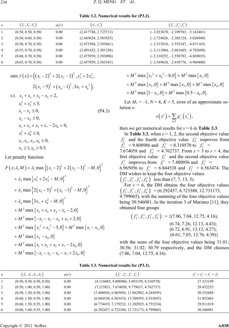

Z. Q. MENG ET AL.
234
Table 3.2. Numerical results for (P3.2).
s 
123
,,
s
ss

 e(xs)


12
,
s
s
x
x


123
,,
s
ss
f
ff
1 (0.50, 0.50, 0.50) 0.00 (2.417748, 2.725713) (–3.033678, –2.109783, –5.143461)
2 (0.50, 0.60, 0.50) 0.00 (2.443024, 2.583925) (–2.724826, –2.302124, –5.026949)
3 (0.50, 0.70, 0.50) 0.00 (2.475504, 2.395661) (–2.315818, –2.555347, –4.871165)
4 (0.55, 0.70, 0.50) 0.00 (2.491432, 2.301258) (–2.111084, –2.681605, –4.792690)
5 (0.60, 0.70, 0.50) 0.00 (2.475939, 2.393096) (–2.310252, –2.558783, –4.869035)
6 (0.65, 0.70, 0.50) 0.00 (2.457059, 2.503341) (–2.549624, –2.410776, –4.960400)
 



22
22
123
22
2
567
2345
22
12
13
24
12578
22
78
1256
min223 ,2,
251,3,
s.t. 2,
5,
0,
0,
20,
8,
,,,0,



  

222 2
78 1
222
25
22
38
max8,0max,0
max, 0max, 0max, 0
max1,0max0.5,0.
Mxx Mx
MxMxMx
MxMx



4
8
f
xxx xx
xxxx
xxxx
xx
xx
xx
xx xxx
xx
xx xx

 




 


38
1,0.5.xx
(P4.3)

6
Let M1 = –1, N = 4, K = 5, error of an approximate so-
lution x:


*s

j
s
iI
exg x




,
then we get numerical results for s = 6 in Table 3.3.
Let penalty function
 








2
22
112
2
22
234
2
22
356
2
2
478
2
2345
2
2345
222 2
12 1
;,max2 23,0
max2,0
max251,0
max3,0
max2,0
max2,0
max5,0max
Fx MxxM
xxM
xxM
xxM
Mxxxx
Mxxxx
Mxx Mx















3
2
24
2
1257 8
2
1257 8
,0
max,0
max2,0
max2,0
x
Mxx
Mxxxxx
Mxxxxx




In Table 3.3, when s = 1, 2, the second objective value
2
s
f
and the fourth objective value 4
s
f
improves from
2
s
f
= 9.808986 and 4
s
f
= 8.310570 to 2
s
f
=
7.674058 and 4
s
f
= 4.762737. From s = 3 to s = 4, the
first objective value 1
s
f
and the second objective value
2
s
f
improves from 1
s
f
= 7.480056 and 2
s
f
=
6.965056 to 1
s
f
= 6.844538 and 2
s
f
= 6.563474. The
DM wishes to keep the four objective values


213 4
,,,
s
sss
f
fff less than (7, 7, 13, 5).
For s = 6, the DM obtains the four objective values


213 4
,,,
s
sss
f
fff = (6.292457, 6.723388, 12.731173,
4.799065), with the summing of the four objective values
being 30.546081. In the iteration 3 of Mariano [11], they
obtained four groups


213 4
,,,
s
sss
f
fff : = {(7.06, 7.04, 12.75, 4.16);
(6.74, 7.26, 12.13, 4.43);
(6.72, 6.91, 13.12, 4.27);
(6.61, 7.03, 12.76, 4.39)}

with the sums of the four objective values being 31.01;
30.56; 31.02; 30.79 respectively, and the DM chooses
(7.06, 7.04, 12.75, 4.16).
Table 3.3. Numerical results for (P3.3).
s

1234
,,,
ssss


e(xs)


1234
,,,
ssss
f
fff 1234
s
sss
f
fff
1 (0.50, 0.50, 0.50, 0.50) 0.00 (4.110485, 9.808986, 5.093159, 8.310570) 27.323199
2 (0.50, 1.00, 0.50, 1.00) 0.00 (7.215821, 7.674058, 9.779637, 4.762737) 29.432253
3 (0.50, 1.50, 0.50, 1.00) 0.00 (7.480056, 6.965056, 11.862982, 4.244595) 30.552688
4 (0.60, 1.50, 0.50, 1.00) 0.00 (6.844538, 6.563474, 13.309395, 4.335055) 31.052463
5 (0.60, 1.50, 0.55, 1.00) 0.00 (6.774419, 7.179232, 11.202925, 4.755234) 29.911810
6 (0.60, 1.60, 0.55, 1.00) 0.00 (6.292457, 6.723388, 12.731173, 4.799065) 30.546081

235 Z. Q. MENG ET AL.
4. Conclusions
In this paper, using the nonlinear penalty function method
with objective parameters, we present an interactive al-
gorithm to solve the multi-objective programming with
inequality constraints. With this algorithm, we can read-
ily find out a satisfactory solution. When objective pa-
rameter M is increased, we may obtain a stable solution,
but unsatisfactory. Then, by adopting different weights in
the algorithm, we can go on interacting with computer
and get many approximate different solutions, among
which we can choose a satisfactory one. By the objective
penalty function, new algorithms for multiobjective pro-
gramming and bilevel multiobjective programming de-
serve further study.
5. Acknowledgements
This research is supported by the National Natural Sci-
ence Foundation of China under grunt 10971193 and the
Natural Science Foundation of Zhejiang Province with
grant Y6090063. We thank the referees for their helpful
comments on a previous version of the paper.
6. References
[1] R. Benayoun, J. de Montgoler, J. Tergny and O. Larichev,
“Linear Programming with Multiple Objective Functions:
Stem Method (STEM),” Mathematical Programming,
Vol. 1, No. 3, 1971, pp. 355-375.
doi:10.1007/BF01584098
[2] A. M. Geoffrion, J. S. Dyer and A. Feinberg, “An Inter-
active Approach for Multi-Criterion Optimization, with
an Application to the Operation of an Academic Depart-
ment,” Management Science, Vol. 19, No. 4, 1972, pp.
457-368. doi:10.1287/mnsc.19.4.357
[3] S. Zionts and J. Wallenius, “An Interactive Programming
Method for Solving the Multiple Criteria Problem,”
Management Science, Vol. 22, No. 6, 1976, pp. 652-663.
doi:10.1287/mnsc.22.6.652
[4] E. E. Rosinger, “Interactive Algorithm for Multiobjective
Optimization,” Journal of Optimization Theory and Ap-
plications, Vol. 35, No. 3, 1981, pp. 339-365.
doi:10.1007/BF00934907
[5] S. Zionts and J. Wallenius, “An Interactive Multiple for a
Class of Underlying Nonlinear Utility Functions,” Man-
agement Science, Vol. 29, No. 5, 1983, pp. 519-529.
doi:10.1287/mnsc.29.5.519
[6] S. Sadagopan and A. Ravinderan, “An Interactive Algo-
rithm for Multiple Citeria Nonlinear Programming Prob-
lems,” European Journal of Operational Research, Vol.
25, No. 2, 1986, pp. 247-257.
doi:10.1016/0377-2217(86)90089-5
[7] S. Helbig, “An Interactive Algorithm for Nonlinear Vec-
tor Optimization,” Applied Mathematics and Optimiza-
tion, Vol. 22, No. 1, 1990, pp. 147-151.
doi:10.1007/BF01447324
[8] M. Abd El-Hady Kassem, “Interactive Stability of Mul-
tiobjective Nonlinear Programming Problems with Fuzzy
Parameters in the Constraints,” Fuzzy Sets and Systems,
Vol. 73, No. 2, 1995, pp. 235-243.
doi:10.1016/0165-0114(94)00317-Z
[9] B. Aghezzaf and T. Ouaderhman, “An Interactive Interior
Point Algorithm for Multiobjective Linear Programming
Problems,” Operations Research Letters, Vol. 29, No. 4,
2001, pp. 163-170. doi:10.1016/S0167-6377(01)00089-X
[10] M. A. Abo-Sinna and T. H. M. Abou-El-Enien, “An In-
teractive Algorithm for Large Scale Multiple Objective
Programming Problems with Fuzzy Parameters through
TOPSIS Approach,” Applied Mathematics and Computa-
tion, Vol. 177, 2006, pp. 515-527.
doi:10.1016/j.amc.2005.11.030
[11] M. Luque, F. Ruiz and R. E. Steuer, “Modified Interac-
tive Chebyshev Algorithm (MICA) for Convex Multiob-
jective Programming,” European Journal of Operational
Research, Vol. 204, No. 3, 2010, pp. 557-564.
doi:10.1016/j.ejor.2009.11.011
[12] Z. Q. Meng, Q. Y. Hu and C. Y. Dang. “A Penalty Func-
tion Algorithm with Objective Parameters for Nonlinear
Mathematical Programming,” Journal of Industrial and
Management Optimization, Vol. 5, No. 3, 2009, pp. 585-
601. doi:10.3934/jimo.2009.5.585
[13] F. H. Clarke, “Optimization and Nonsmooth Analysis,”
John-Wiley & Sons, New York, 1983.