 American Journal of Oper ations Research, 2011, 1, 191-202 doi:10.4236/ajor.2011.14022 Published Online December 2011 (http://www.SciRP.org/journal/ajor) Copyright © 2011 SciRes. AJOR 191 Optimal Adjustment Algorithm for p Coordinates and the Starting Point in Interior Point Methods Carla T. L. S. Ghidini1, Aurelio R. L. Oliveira1, Jair Silva2 1Institute of Mathematics, Statistics and Scientific of Computation (IMECC), State University of Campinas (UNICAMP), São Paulo, Brazil 2Federal University of Mato Grosso do Sul (UFMS), Mato Grosso do Sul, Brazil E-mail: {carla, aurelio}@ime.unicamp.br, jairmt@gmail.com Received September 15, 2011; revised October 16, 2011; accepted October 30, 2011 Abstract Optimal adjustment algorithm for p coordinates is a generalization of the optimal pair adjustment algorithm for linear programming, which in turn is based on von Neumann’s algorithm. Its main advantages are sim- plicity and quick progress in the early iterations. In this work, to accelerate the convergence of the interior point method, few iterations of this generalized algorithm are applied to the Mehrotra’s heuristic, which de- termines the starting point for the interior point method in the PCx software. Computational experiments in a set of linear programming problems have shown that this approach reduces the total number of iterations and the running time for many of them, including large-scale ones. Keywords: Von Neumann’s Algorithm, Mehrotra’s Heuristic, Interior Point Methods, Linear Programming 1. Introduction In 1948, von Neumann proposed to Dantzig an algorithm for finding a feasible solution to a linear program with a convexity constraint recast in the form ([1,2]): Px = 0, etx = 1, (1.1) 0x where , , is the vector of all ones, and the columns of P have norm one, i.e., Rmn P Rn xRn e 1 j P , for . 1, ,jn This algorithm, which was later studied by Epelman and Freund [3], has interesting properties such as sim- plicity and fast initial advance. However, it is not very practical for solving linear problems because its conver- gence rate is slow. Gonçalves [4] presented four new algorithms based on von Neumann’s algorithm and among them the optimal pair adjustment algorithm has the best performance in practice. The optimal pair adjustment algorithm inherits the good properties of von Neumann’s algorithm. Although it is proved in [5] that this algorithm is faster than von Neumann’s algorithm, nevertheless, it is impractical to solve linear programming problems, because its conver- gence rate is also very slow. In [6], the idea presented by Gonçalves, Storer and Gondzio [5] to develop the optimal pair adjustment algo- rithm was generalized for p coordinates and then the op- timal adjustment algorithm for p coordinates arose. The value of p is bounded by the number of variables of the problem. The new algorithm is not suitable to solve linear pro- gramming problems until achieving optimality. Thus, the idea is to exploit its simplicity and quick initial progress during the early iterations and to use it together with an interior point method to accelerate convergence. Knowing that the starting point greatly influences the performance of the interior point method, in this work the optimal adjustment algorithm for p coordinates is applied within the Mehrotra’s heuristic [7], which deter- mines the starting point for the method interior points in the PCx software, so that the starting points can be ob- tained even better. This approach is different to the clas- sical warm-starting approach, which uses a known solu- tion for some problem (e.g., relaxation in the column- generation) to define a new starting point for a closely related problem or perturbed problem instance ([8-10]). The paper is organized as follows. In Section 2, the definition of the problem is given and von Neumann’s algorithm is described. In Section 3, the optimal pair adjustment algorithm is recalled. In Section 4, the opti- mal adjustment algorithm for p coordinates is proposed  C. T. L. S. GHIDINI ET AL. 192 b k and some theoretical results are described. Section 5 dis- cusses warm-starting in interior point methods. Numeri- cal experiments are shown in Section 6. In Section 7, the conclusions are drawn and future perspectives are sug- gested. 2. Von Neumann’s Algorithm Considering the problem of finding a feasible solution of the set of linear constraints (1.1), geometrically, the col- umns Pj can be viewed as points lying on the m-dimen- sional hypersphere with unit radius and center at the ori- gin. This problem can be described as assigning non- negative weights xj to columns Pj in such a way that after being re-scaled its center of gravity is the origin. First, the algorithm finds the column Ps of P which makes the largest angle with the residue bk-1 = Pxk-1 and then the next residual bk is given by projecting the origin on the line segment connecting bk–1 to Ps. See Figure 1. VON NEUMANN’S ALGORITHM Given: , with etx0 = 1. Compute b0 = Px0. 00x k = 1 Do { 1. Compute: 1 1, , argmintk jnj sP . 11kt s vPb 1k 2. If , then STOP. The problem (1.1) is infea- sible. 0v 3. Compute: 11kk u=b , 1 2 11 1 21 k kk v uv . 4. Update: 11 kk bb P, 11 kk xe . Figure 1. Illustration of von Neumann’ s algorithm. h 1 5. where es is the vector of the canonical basis wit in position s. Stopping Criterion: 1kkk k E=b bb k = k + 1. } ε)}, here ε is a predetermined percentage. e initial approxi- m while (Ek > w Note that bk = Pxk, for all 0k. Th ation x0 is arbitrary, since e 1, then xj = 1/n for 1, ,jn tx0 = was used. For any given iteration k column lumn which makes the largest angle with the vector bk−1. Furthermore, if 11 0 ktk s vPb , then 0 < 1 − vk−1 < (uk−1)2 − 2vk−1 + 1 threover, the new residual is smaller than the previous one, i.e., uk < uk−1, as can easily be seen in Figure 1, the triangle 0bk−1bk has hypotenuse uk−1 = 0bk−1 and side uk = 0bk. The effort per iteration of von Neumann’s algorithm is Ps is the co us, 0 < λ < 1. Mo do . Optimal Pair Adjustment Algorithm his PhD thesis [4], Gonçalves studied von Neumann’s ithm was proposed as an at xpected that the new residual bk is cl onds to making residual bk−1 move in the di ubject to minated by matrix-vector multiplication needed when selecting column Ps which is O(nz(P)) where nz(P) is the number of the entries of P. This effort can be reduced significantly as the matrix P is sparse. For more details of this algorithm see [11,12]. 3 In algorithm and introduced four new algorithms based on it. Among them, emphasis is given to the weight-reduc- tion algorithm and the optimal pair adjustment algorithm. The optimal pair adjustment algorithm was the one that performed better in practice. The weight-reduction algor tempt to improve the efficiency of von Neumann’s algorithm. It is based on the idea that the residual bk−1 can be moved closer to origin 0, increasing the weight xj for a given column Pj and decreasing the weight xi for another column Pi. In particular, it is e oser to origin 0 than the residual bk−1 if the weight in column Ps+ is increased when Ps+ has the largest angle with the residual bk−1 and the weight in column Ps− is decreased when Ps+ has the smallest angle with the re- sidual bk−1. This corresp rection Ps+ − Ps−. The new residual bk is the point that minimizes the distance from origin 0 to this line. Notice that the minimization of this distance is s the maximum possible decrease of xs−. Since 0 j x for all j, then xs− can be decreased until it vanishe ure 2 is a geometric illustration of how the algorithm works by iteration. s. Fig- Copyright © 2011 SciRes. AJOR  193 C. T. L. S. GHIDINI ET AL. Figure 2. Illustration of weight-reduction algorithm. 3.1. Optimal Pair Adjustment Algorithm he optimal pair adjustment algorithm is a generalization algorithm, the optimal pa T of the weight-reduction algorithm designed to give the maximum possible freedom to two of the weights xj (see [5]). In a way, we can say that it prioritizes only two variables by iteration because it finds the optimal value for two coordinates and adjusts the remaining coordi- nates according to these values. Similar to the weight-reduction ir adjustment algorithm starts by identifying vectors Ps+ and Ps− , which make the largest and smallest angles with the vector bk−1. Afterwards, values k , k , are found, where 1kk j x for all js js . These vaize the distance between origin while satisfying the convexity and the non-negativity constraints. The solution of this optimiza- tion problem is easily computed examining the Karush- Kuhn-Tucher conditions (KKT). The main difference between th and lues minimbk and the e weight-reduction al- go OPTIMAL PAIR ADJUSTMENT ALGORITHM Giv 1. Compute: Pb rithm and the optimal pair adjustment algorithm is that only the weights of Ps+ and Ps− are changed in the first algorithm while in the second algorithm all other weights are also changed. en: 00x, with etx0 = 1. Compute b0 = Px0. k = 1 Do { 1 1,..., ntk jnj , argmis 1 1,..., argmax0 tk jnjj sPbx , 2. If , then STOP. The problem (1.1) is infea- 3. he problem: 11ktk s v=Pb 1k0v le. sib Solve t 2 min b 11 01 2 s.t. 11, 0, for 0,1,2. kk ss i xx i (3.2) where 11 1 012 kk k ssss s bxP xPPP b . 4. Update: 11 1kk k 0 k 1 2 ssss s bxP xPPP b , kk u=b , 1 0 1 2 , and , , j k k js js x=j s js 5. Stopping Criterion: 1kkk k E=b bb k = k + 1. } ε)}. In iteration k, column Ps+ is the column which makes th .2. Subproblem Solution order to solve subproblem (3.2), first the subproblem while (Ek > e largest angle with the vector bk−1 and column Ps− is the column which makes the smallest angle with the vector bk−1 such that xs > 0. 3 In is rewritten as: 2 12 min s.t. 10, 0, for 0,1,2. i b i (3.3) where, 11 1 12 1 11 2 1 1 . kk k sss s kk ss s bbxPxP xx P P Define: g1 + λ2 − 1, g1(λ1 , λ2) = −λ1, g2(λ1 , λ2) = −λ2. 0(λ1, λ2) = λ Denote the objective function by f(λ1, λ2) and let 12 , be a feasible solution. dering the convexity of theConsi objective function and constraints, if 12 , is an optimal local solution then it is also an oplobal solution. Thus, timal g 12 , met the KKT constraints given by: 2 12 12 0 ,, ii i fg 0. Copyright © 2011 SciRes. AJOR  C. T. L. S. GHIDINI ET AL. 194 12 12 (,)0,for 0,1,2. (,)0,for 0,1,2. 0,for 0,1,2. i ii i gi gi i where µi are Lagrange multipliers. Problem (3.3) is solved by selecting a feasible solution 1; λ1 + λ2 − 1 = 0; re replaced in thear system is so inates s eg the ideas used in [5] for the op- COORDINATES it00 0 k = ompute: among all possibilities that meet the KKT conditions. This is done by analyzing the following cases: a) λ1 = λ2 = 0; b) λ1 = 0; 0 < λ2 < 1; c) λ1 = 0; λ = 1; 2 d) 0 < λ < 1; λ 1 2 = 0; e) 0 < λ < 1; 0 < λ2 < 1 f) λ = 1; λ = 0; 1 2 g) 0 < λ < 1; 0 < λ < 12 1; λ1 + λ2 − 1 = 0; ove, the known values aFor each case ab e KKT equations and the resulting lin lved. 4. Optimal Adjustment Algorithm for p Coord The optimal adjustment algorithm for p coordinates i veloped generalizind timal pair adjustment algorithm. Instead of only two columns to be used to formulate the problem, any amount of columns can be used and thus, importance will be given to any desired amount of variables. The strategy to prioritize the variables is free. In this work, we chose to take p/2 columns making the largest angle with the vector bk and the remaining p/2 columns that make the smallest angle with the vector bk. If p is odd then one more column is added to the set of vectors that make the largest angle with the vector bk, for exam- ple. The structure of the optimal adjustment algorithm for p coordinates is similar to the optimal pair adjustment algorithm. It begins by identifying the s1 columns that make the largest angle with the vector bk−1, then s2 col- umns that make the smallest angle with the vector bk−1 are determined, where s1 + s2 = p and p is the number of columns that are prioritized. Next, the optimization sub- problem is solved and the residual and the current point are updated. OPTIMAL ADJUSTMENT ALGORITHM FOR p G ven: 0x, with ex = 1. Compute b = Px . 1 0 Do { 1. C 11 P, ,P s −1 , which make the largest angle with . the vetor bk 11 P, ,P s such that , where s1 + s2 = p. , which make the smallest angle with the vector bk−1 and 10 k i x 11kt 1k 1 1, , minim um i is vPb If v k 2. , then STOP. The problem (1.1) is infea- 3. Solve the problem: 0 sible. 1 1 s.t. 1 s k x 2 12 2 1 0 11 11 0 1 2 1, 0, 0, for 1,,, 0, for 1,,. ij ij i j s ss k ij ij x is js min b (4.4) where 12 1 2 11 1 0 11 1 1 ii jjii jj ss s kk k ij i j bb xPxPP P s 4. Update: P 12 1 2 11 1 0 11 1 1 , ii jjii jj ss s kkk k ij i j bbxPxP P s kk u=b , 12 1 011 1 2 ,,,,,,, ; 1,,, ,; 1,,. i k jss k ji j j xj xji s jj s , 5. Stopping Criterion: 1kkk k E=b bb k = k + 1. while (Ek > ε)}. } f the algorithm, if vk−1 > 0 then all columns Pj n the same side of the hyper-plane rough the origin and perpendicular to direction bk−1. This m resulting in the origin can be found. In this case, the In Step 2 o of matrix P are o th eans that any convex combination of the columns Pj Copyright © 2011 SciRes. AJOR  C. T. L. S. GHIDINI ET AL. 195 or each iteration of the optimal adjustment algorithm m (4.4lem is solved finding a solution in the ositive orthant, subject to a linear equation system of problem is infeasible. 4.1. Subproblem Solution Using Interior Point Methods F for p coordinates, it is necessary to solve subproble ). This subprob p order (p + 1). A way to solve it is to verify all possible feasible solutions as in the pair adjustment algorithm. The drawback that comes naturally in solving the sub- problem in this way is that the number of possible cases to be verified grows exponentially with the value of p as shown next. In fact, to solve the subproblem (4.4) first the variable λ0, as defined in (4.5), is removed from the problem. 12 ss 12 11 0 11 1 ij ij ss kk 11 1 ij ij x (4.5) Thus, the subproblem (4.4) was rewritten as: 12 2 11 1 2 min s.t. 10, ij 0, for 1,,, 0, for 1,,. i j ss ij b is js (4.6) where 12 1 2 11 1 0 11 1 1 ii jjii jj ss s kkk ij i s j b bxPxPP P Defining: 12 11 2 1 0 11 ,,, ,,1 sij s ss ij g 11 2 1 1 ,,,,,, 1,, si s i is 11 2 1 2 ,,, ,,,1,, sj s j h j and denoting the objective function by , the KKT conditions oe subproblem are given by: s 11 2 1 ,,,,, s s f f th 11 1 1 1 2 1 2 11 2 1 11 2 1 11 1 0 0 1 ,,,,, , ,, ,,, ,,0, ,,,,,0, for 0,,, ,,, , s s s js s is s js s s hj j gi hj f h 2 s 1 ,, i gi i g is h 2 11 2 1 11 2 1 2 1 2 1 2 ,0, for 1,,, 0, for 0,,, 0, for 1,,, ,,,,,0, for 0,,, ,,,,,0, for 1,,. s i j s s s s g h i j js is js gi hj s s (4.7) Then, the subproblem (4.6) is solved by selecting a feasible solution among all the possibilities that satisfy the KKT conditions (4.7). For this, all possible cases of possible values for the variables i , 1 1, ,is , and , 2 1, ,js , must be analyzed. The cases to be considered are: Case: 0 i , 1 1, ,is and 0 j , 2 1, ,js , Case: one 0 k , with 12 11 ,, ,,, ss k and others equal to zero, which gives a combination of 1 C cases, but again we have to conside case where 1 k r the and 1 k . Thus, we have 1 2 C possi Case: 0 i bilities. and 0 j , and 12 11 ,,,,,, ss ij and others equal to zero, which gives a combination of 2 C cases, but again we have to consider the case where 1 ij and 1 ij . Thu possibilities. The total number of cases when p coordinates are modified is: 1 123 12222 21 p ppp p CCCC s,ve we ha p C2 2 p erefore, this straThtegy is inefficient even for values of p which are not too large. In order to deal with such a difficulty, the subproblem (4.4) is approached differently and solved using interior point methods. This is done as follows: First, the subproblem is rewritten in matrix form: Copyright © 2011 SciRes. AJOR  C. T. L. S. GHIDINI ET AL. 196 2 1 min 2 s.t. 1, t W a 0, (4.8) where 11 2 s 1 12 11 2 1 12 11 1 11 0 11 11 11 , , ,,,,,, , 11, 1 s ii jj s s ij ss kkk ij t ss tkk ij WwPPPP wbxP xP aaaxx (4.9) The KKT equations of problem (4.8) are given (4.10) where, γ and µ are Lagrange multipliers of equality and in 1) is Now the interior point method is applied to those equations. by: 0, 0, 10, 0, 0. ttt WW aa equality constraints respectively and (p + 1) × (p + the dimension of the matrix WtW. The linear system arising at each iteration of the inte- rior point method applied to (4.10) are: d t WW aI 1 2 0dUr 3 00d t ar r where (4.11) Udiag , diag , 1 t raWW , 2 t r , 31t ar . By performing some algebraic manipulations, the di- dµ, dλ and dγ are given by: 1 (4.12) where r4 = r1 + Λ–1r2. Defining sl1 = (WtW + Λ–1U)–1 a and sl2 = (Wt Λ–1U)–1r4, to compute the directions the following linear systems must be solved: , 4.2. Theoretical Properties of the Optimal bed below and proved in [6], nsure that the optimal adjustment algorithm for p coor- e con- vergat, om the theoretical point of view, for larger values of p rections 11 2 1 11 4 43 dd, d d, tt µrU WW UrWWUa 11 11 d, tt tt aW WU aaWWU rr W + (4.13) –1 1 t WWU sla –1 4 2 t WWU slr Note that (WtW + Λ–1U) is a positive definite matrix of order p + 1 and both systems can be solved using the same factorization. Adjustment Algorithm for p Coordinates Theorems 1 and 2, descri e dinates converge in the worst case with the sam ence rate of von Neumann’s algorithm and th fr the algorithm is more robust and will perform better. Theorem 1 The decrease in k b obtained by an it- eration of the optimal adjustment algorithm for p coor- dinates, with 1pn , where n is the column number of matrix P, in the worst case, is equal to the decrease obtained by an iteration of von Neumann’s algorithm. Theorem 2 The decrease in k b obtained by an it- eration of the optimal adjustment algorithm for p2 coor- dinates, in the se is equal to that obtained by an iteration of the optimal adjustment algorithm for p1 co- ordinates with 12 ppn worst ca , where n is the P column nu p. Howeve that the starting point can influence the erformance of interior point methods. On the other hand, s a son, a natural idea is use this algorithm to find a good starting point for in- mber. On the other hand, it is not advisable to choose a very large value of p since there is a cost of building and up- dating matrix W in (4.13). Such a cost is negligible for small values of r, it becomes noticeable for larger values. 5. Mehrotra’s Heuristic and Starting Point in Interior Point Methods It is well known p as the optimal adjustment algorithm for p coordinates ha mall computational cost per iterati to terior point methods or improve the current one. In this work, few iterations of the optimal adjustment algorithm for p coordinates are performed to improve the starting point introduced by Mehrotra’s heuristic [7]. This heuris- tic consists of the following steps: 1) Use least squares to compute the points: 1 t y= AAAc , t z=cAy , 1 tt =A AAb where x, y and z are the primal variables, dual variables and dual slacks respectively. 2) Find values δx and δz such that x an z d are non-negative: max1.5 min, 0 , xi x max1.5 min, 0 . zi z 3) Determine and suc0 h that the points x and Copyright © 2011 SciRes. AJOR  C. T. L. S. GHIDINI ET AL. Copyright © 2011 SciRes. AJOR 197 z0these are improved. However, the centrality, which is important for the interior point methods, may be lost. are centralized: 1 iz 2 t xz xx n i ez e z , We have adapted the optimal adjustment algorithm for p coordinates in the PCx code [13] aiming to improve the starting point given by Mehrotra [7]. The starting point for the optimal adjustment algo- rithm for p coordinates is determined by solving the least squares in Step 1. 1 2 t xz zz n ix i ez e x . 6. Computational Experiments 4) Compute the starting points as follows: 0 =y , 0 zz e , 0 xe . Remark 5.1 Any linear programming problem can be reduced to problem (1.1 ). For details of this transforma- tio Usually, to imove the perfmance of inior point methods, modifications are introd after Step 4 of the al orithm for p coordinates before centraliz- in st problems. Rows Columns Problem Rows Columns In the following experiments, all testing was performed on an Intel Core 2 Duo T7250, 2 GB RAM, 2 GHz and 250 GB hd and Ubuntu 32-bit operating system. We used 76 test problems to compare the performance of the original PCx and the modified PCx (PCxMod), which uses the optimal adjustment algorithm for p coordinates as a warm-starting approach. Most tested problems have free access such as NETLIB problems, QAPLIB prob- lems and KENNINGTON problems ([14,15]). Other problems, which are not available publicly, were ob- tained from Gonçalves [4]. The test problems are pre- sented in Table 1. n see [4]. pror ter duce gorithm described above, unlike our proposal, which consists of performing a few iterations of the optimal adjustment alg g, i.e., before Step 2. One explanation for this is that if the algorithm is then used after to centralize the points, Table 1. Te Problem Rows Columns Problem NETLIB Miscellaneous Gonçalves 80bau3b 2140 11066 nug06 agg2 514 750 nug07 372 486 bl 5729 12462 602 931 bl2 5729 12462 agg3 514 750 nu1632 co5 4849 10787 czprob 671 2779 c6692 co9 9090 19997 dfl001 12143 cre-c 5412 ex01 1556 2 ex02 f 1 1 1 2 1 m f m pilot87 1971 6373 p stocfor3 2 13 g08 912 re-a 2994 degen3 1503 2604 cre-b 5336 36382 cq9 8004 19317 5984 2375 235 etamacro 334 669 cre-d 4102 8601227 1548 ffff800 322 826 ken-11 0085 6740ex05 832 7805 fit2d 25 0524ken-13 2534 36561 ex06 825 7797 fit2p 3000 13525 ken-18 78862 28434ex09 1821 18184 aros-r7 2152 7440 osa-07 1081 25030 ort45 1152 1582 odszk1 665 1599 osa-14 2300 54760 fort47 1152 1582 perold 593 1389 osa-30 4313 104337 fort48 1152 1582 pilot 1368 4543 osa-60 10243 243209 fort53 1156 1586 els19 4350 13186 fort56 1156 1586 ilotwe 701 2814 chr25a 8149 15325 fort58 1156 1586 scfxm3 915 1704 chr22b 5587 10417 fort59 1156 1586 seba 448 901 scr15 2234 6210 fort60 1156 1586 ship08l 470 3121 scr20 5079 15980 fort61 1156 1586 15362 22228 rou20 7359 37640 ge 9150 14990 wood1p 171 1718 pds-02 2609 7339 nl 6665 14680 pds-20 32287 106080 x1 1050 1480 pds-30 47968 156042 x2 1050 1480 pds-40 64276 14385 pds-50 80339 272513 pds-60 96514 332862 pds-70 11896 86238 pds-80 126120 430800 pds-90 139752 471538 pds-100 152300 498530  C. T. L. S. GHIDINI ET AL. 198 6.1. Choice of p For the timal adjustent algorithm for p cos to work properly an apopriate choice of parap is ssentia Thus, several computational experiere heuristic that works well in any lin- roblem. With results obtained in the op mordinate pr meter e l.ments w done to determine a ear programming p tests, it became clear that the value of p must be chosen depending on the size of the problem. Recalling that m is the number of rows and n is the number of columns of the linear problem constraint matrix, the heuristic that showed better results is as follows: 0 < (m + n ) ≤10,000 → p = 4; 10,000 < (m + n ) ≤20,000 → p = 8; 20,000 < (m + n ) ≤400,000 → p = 20; 400,000 < (m + n ) ≤600,000 → p = 40; 600 0,00 < (m + n ) → p = 80. 6.2. Stg The nfrfel slgo- rithm oibrfmedartant be determsince it directly influences x. This algorithm achieves tion is determined with good d in Table 2. nterior point iterations (Column the total running time in seconds (Column e PCxMod takes less time obtaiptimal solution in 55.3% of the tested bleme PCx in 34.2% of te problemsore- r, theber of iterations was lower in 40.8% the ps for the PCxMod a d 1.3% (only one hose are the most important problems to be were solved only by PCxMod. iterion previously described was deter- m .5% of th red. given po he reso- lu the tested problems. Considering the pds-80 pr stment algorithm for p co- oppin Criterion umber o iteations o th optimaadjutment a for p c eter to ordnates to ined, e peor is n impo param the performance of the PC better results when the solu accuracy. However, in some cases, the number of itera- tions needed for convergence of the algorithm can be very large, making it impractical to use. In these cases, a maximum number of iterations should be adopted. There- fore, the stopping criterion for the optimal adjustment algorithm for p coordinates used is the following: maxi- mum number of iterations (100) or the relative error of the residual norm smaller than a given tolerance (10−4) (the one that occurs first). 6.3. Results The performance of the PCx and PCxMod was compared with respect to the total number of iterations and the run time. The results are presente The total number of i Iterations) and Time) of two versions of the PCx are showed in Tab le 2. The PCxMod is the version that uses the optimal adjust- ment algorithm for p coordinates in Mehrotra’s heuristic and PCx is the one that does not adopt it. Column p shows the value of p used by the optimal adjustment al- gorithm. Column ItAux gives the number of iterations performed by the optimal adjustment algorithm for p coordinates. problem) for the PCx. In this case, the run time of the PCxMod was lower because a better starting point was used. In almost all problems with larger running time, the new approach performed better than the traditional one. This reveals a welcome feature of the proposed ap- proach, since t According to the results, th to n the o pros and th h. M ove total num of roblem n solved. Although the total number of iterations did not de- crease in some problems, a better starting point was de- termined as the optimal adjustment algorithm for p coor- dinates was used after Step 1 of the Mehrotra’s heuristic and, consequently, the running time was reduced. An interesting result is the fact that two problems (co9 and nug08) In another experiment, the same set of test problems were solved using only the PCxMod. First, p = 2 (2-co- ord) was considered, which represents the optimal pair adjustment algorithm and after the value of p according to the stopping cr ined. The results obtained are shown in Table 3. The results showed that the PCxMod takes less itera- tions with values of p greater than 2 in 40.8% of the tests problems. For p = 2 this number is approximately 5.3%. The total running time was reduced by about 60 e problems for p-coordinates and only 22.4% were solved in a lower time as p = 2 was conside Again the problem co9 obtained status optimal only for p = 8. These tests confirmed that the performance of the al- gorithm is improved by increasing the value of p. That happens because the residual bk has a greater reduction from one iteration to another and also because the int by the algorithm as a solution is different for each value of p. The obtained points for p > 2 achieved better performance in most cases. It should be mentioned that the required total time to obtain a solution for the optimal adjustment algorithm for p coordinates is not significant in relation to t tion total time of the problems. This time is almost null in many of oblem, the time spent by the optimal adjustment algo- rithm was 24 seconds, which represents approximately 0.07% of the total running time. 7. Conclusions and Future Work In this work, the optimal adju Copyright © 2011 SciRes. AJOR 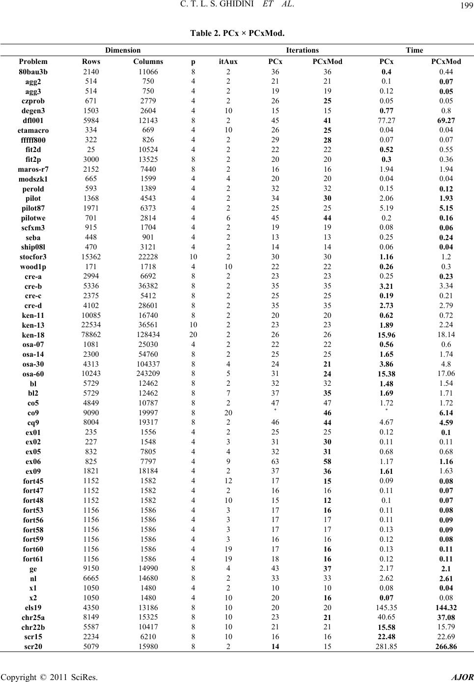 C. T. L. S. GHIDINI ET AL. 199 x × e Table 2. PC PCxMod. Dimension Iterations Tim Problem Rows Columns p itAux PCxMod PCx PCxMod PCx 80bau3b 2140 11066 8 2 agg2 514 750 4 2 agg3 514 750 4 2 czprob 671 2779 4 2 degen3 1503 2604 36 36 0.4 0.44 21 21 0.1 0.07 19 19 0.12 0.05 26 25 0.05 0.05 15 0.77 0.8 dfl001 5984 12143 41 77.27 69.27 etam 334 669 10 26 25 0.04 0.04 m7 m 1 1 2 1 2 f f f 1 1 2 2 4 10 15 8 2 45 acro 4 fffff800 322 826 4 2 29 28 0.07 0.07 fit2d 25 3 10524 1 4 2 22 22 0.52 0.55 fit2p 00035258 2 20 20 0.3 0.36 aros-r 2152 7440 8 2 16 16 1.94 1.94 odszk1 665 1599 4 4 20 20 0.04 0.04 perold 593 1389 4 2 32 32 0.15 0.12 pilot 1368 4543 4 2 34 30 2.06 1.93 pilot87 1971 6373 4 2 25 25 5.19 5.15 pilotwe s701 2814 4 6 45 44 0.2 0.16 cfxm3 915 1704 4 2 19 19 0.08 0.06 seba 448 901 4 2 13 13 0.25 0.24 ship08l 470 1 3121 4 2 14 14 0.06 0.04 stocfor3 wood 5362 22228 10 2 30 30 1.16 1.2 1p 171 1718 4 10 22 22 0.26 0.3 cre-a 2994 6692 8 2 23 23 0.25 0.23 cre-b 5336 36382 8 2 35 35 3.21 3.34 cre-c 2375 5412 8 2 25 25 0.19 0.21 cre-d k 4102 28601 8 2 35 35 2.73 2.79 en-11 00856740 8 2 20 20 0.62 0.72 ken-13 2534 36561 10 2 23 23 1.89 2.24 ken-18 78862 1 128434 2 20 2 26 26 15.96 8.14 osa-07 o0815030 4 2 22 22 0.56 0.6 sa-14 2300 54760 8 2 25 25 1.65 1.74 osa-30 o4313 104337 8 4 24 21 3.86 4.8 sa-60 10243 432098 5 31 24 15.38 17.06 bl 5729 12462 8 2 32 32 1.48 1.54 bl2 5729 12462 8 7 37 35 1.69 1.71 co5 4849 10787 8 2 47 * 47 1.72 * 1.72 co9 9090 19997 8 20 46 6.14 cq9 8004 19317 8 2 46 44 4.67 4.59 ex01 235 1556 4 2 25 25 0.12 0.1 0 ex02 227 1548 4 3 31 30 0.11 .11 ex05 ex06 832 7805 4 4 32 31 0.68 0.68 825 7797 4 9 63 58 1.17 1.16 ex09 1821 18184 4 2 37 36 1.61 1.63 ort45 1152 1582 4 12 17 15 0.09 0. 0.08 ort47 1152 1582 4 2 16 16 110.07 ort48 1152 1582 4 10 15 12 0.1 0.07 fort53 1156 1586 4 3 17 16 0.11 0.08 fort56 1156 1586 4 3 17 17 0.11 0.09 fort58 1156 1586 4 3 17 17 0.13 0.09 fort59 1156 1586 4 3 16 16 0.12 0.08 fort60 1156 1586 4 19 17 16 0.13 0.11 fort61 1156 1586 4 19 18 16 0.12 0.11 ge 9150 14990 8 4 43 37 2.17 2.1 nl 6665 14680 8 2 33 33 2.62 2.61 x1 1050 1480 4 2 10 10 0.08 0.04 x2 1050 1480 4 10 20 16 0.07 0.08 els19 4350 13186 8 10 20 20 45.3544.32 chr25a 8149 15325 8 10 23 21 40.65 37.08 chr22b 5587 10417 8 10 21 21 15.58 15.79 scr15 scr20 2234 5079 6210 15980 8 8 10 2 16 14 16 15 22.48 81.85 22.69 66.86 Copyright © 2011 SciRes. AJOR 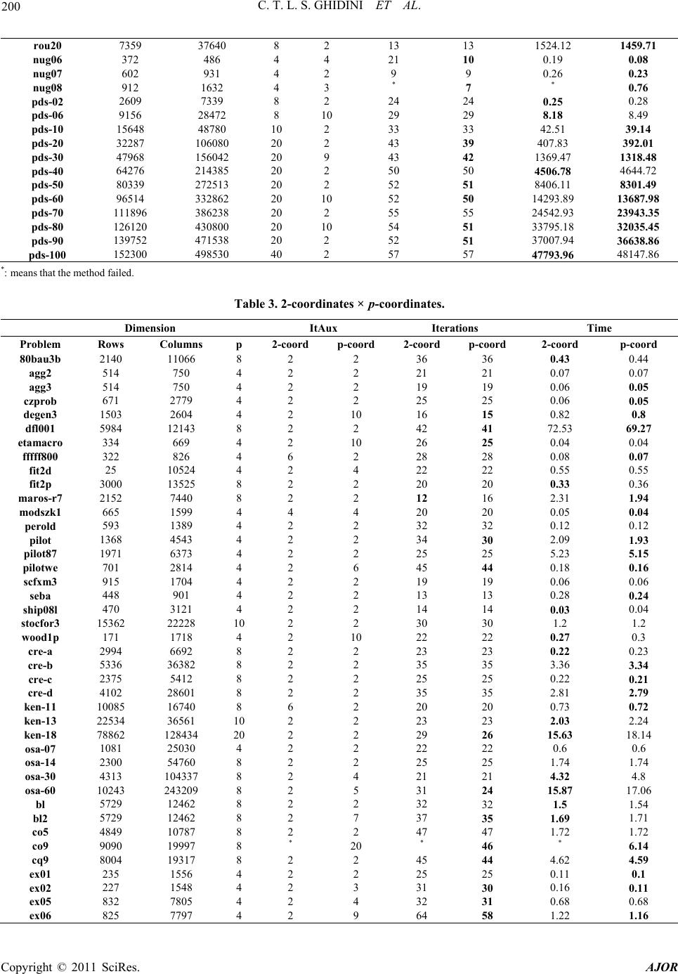 C. T. L. S. GHIDINI ET AL. 200 rou20 1 141 7359 37640 8 2 13 13 524.1259.7 nug06 nug07 nug08 1 8 2 8 8 9 3 149 138 1 3 24593 235 1 4 338 325 1 374 366 4 4 372 486 4 4 21 10 0.19 0.08 602 931 4 2 9 9 0.26 0.23 912 1632 4 3 * 7 * 0.76 pds-02 2609 7339 8 2 24 24 0.25 0.28 pds-06 9156 28472 8 10 29 29 8.18 8.49 pds-10 15648 48780 10 2 33 33 42.51 39.14 pds-20 32287 0608020 2 43 39 407.83 392.01 pds-30 47968 156042 20 9 43 42 1369.47 1318.48 pds-40 64276 214385 20 2 50 50 4506.78 4644.72 pds-50 03397251320 2 52 51 406.11 301.49 pds-60 65143286220 10 52 50 293.8 687.9 pds-70 118968623820 2 55 55 42.943.3 pds-80 261203080020 10 54 51 795.1 035.4 pds-90 39752 471538 20 2 52 51 007.9 638.8 pds-100 152300 498530 40 2 57 57 7793.968147.86 *: mea method fa 3. 2-coordinates × p-cinates. nsion It IteratTime ns that theiled. Table oord DimeAuxions PrRoColump ord p-coord 2-coord oord oblem ws ns 2-cop-c2-coord p-coord 80 2140 11068 2 2 36 36 514 750 4 2 2 21 21 514 750 4 2 2 19 19 2779 4 2 2 25 25 0.06 0.05 degen3 1503 2604 4 2 10 16 15 0.82 0.8 dfl001 5984 12143 41 72.53 69.27 etamacro 334 669 4 2 10 26 25 0.04 0.04 ffff 3226 6 2 280.08 0.07 m7 m ship08l 1 k 2 71 1 bau3b 6 0.43 0.44 agg2 agg3 0.07 0.06 0.07 0.05 czprob 671 8 2 2 42 f800 824 28 fit2d 25 10524 4 2 4 22 22 0.55 0.55 fit2p 3000 13525 8 2 2 20 20 0.33 0.36 aros-r 2152 7440 8 2 2 12 16 2.31 1.94 odszk1 665 1599 4 4 4 20 20 0.05 0.04 perold 593 1389 4 2 2 32 32 0.12 0.12 pilot 1368 4543 4 2 2 34 30 2.09 1.93 pilot87 1971 6373 4 2 2 25 25 5.23 5.15 pilotwe 701 2814 4 2 6 45 44 0.18 0.16 scfxm3 915 1704 4 2 2 19 19 0.06 0.06 seba 448 901 4 2 2 13 13 0.28 0.24 470 3121 4 2 2 14 14 0.03 0.04 stocfor3 15362 22228 10 2 2 30 30 1.2 1.2 wood1p 171 1718 4 2 10 22 22 0.27 0.3 cre-a 2994 6692 8 2 2 23 23 0.22 0.23 cre-b 5336 36382 8 2 2 35 35 3.36 3.34 cre-c 2375 5412 8 2 2 25 25 0.22 0.21 cre-d 4102 28601 8 2 2 35 35 2.81 2.79 ken-11 0085 16740 8 6 2 20 20 0.73 0.72 en-13 2534 3656110 2 2 23 23 2.03 2.24 ken-18 8862 2843420 2 2 29 26 15.63 18.14 osa-07 1081 25030 4 2 2 22 22 0.6 0.6 osa-14 2300 54760 8 2 2 25 25 1.74 1.74 osa-30 4313 043378 2 4 21 21 4.32 4.8 osa-60 10243 243209 8 2 5 31 24 15.87 17.06 bl 5729 12462 8 2 2 32 32 1.5 1.54 bl2 5729 12462 8 2 7 37 35 1.69 1.71 co5 4849 10787 8 2 2 47 47 1.72 1.72 co9 9090 19997 8 * 20 * 46 * 6.14 cq9 8004 19317 8 2 2 45 44 4.62 4.59 ex01 235 1556 4 2 2 25 25 0.11 0.1 ex02 227 1548 4 2 3 31 30 0.16 0.11 ex05 832 7805 4 2 4 32 31 0.68 0.68 ex06 825 7797 4 2 9 64 58 1.22 1.16 Copyright © 2011 SciRes. AJOR  C. T. L. S. GHIDINI ET AL. Copyright © 2011 SciRes. AJOR 201 ex09 1821 18184 4 2 2 37 36 1.67 1.63 f f f 0 f 1 1 3 2 2 rou20 149 141 nug06 nug07 nug08 1 82 8 8 93 148 138 1 3 2235 1 4 327 325 1388 366 4 4 ort45 1152 1582 4 2 12 17 15 0.12 0.08 ort47 1152 1582 4 2 2 16 16 0.12 0.07 ort48 1152 1582 4 2 10 15 12 .060.07 ort53 1156 1586 4 4 3 16 16 0.08 0.08 fort56 1156 1586 4 2 3 17 17 0.1 0.09 fort58 1156 1586 4 2 3 17 17 0.1 0.09 fort59 1156 1586 4 2 3 16 16 0.13 0.08 fort60 1156 1586 4 2 19 17 16 0.14 0.11 fort61 1156 1586 4 2 19 18 16 0.12 0.11 ge 9150 14990 8 2 4 43 37 2.2 2.1 nl 6665 14680 8 2 2 33 33 2.62 2.61 x1 1050 1480 4 2 2 10 10 0.07 0.04 x2 1050 1480 4 2 10 20 16 0.12 0.08 els19 4350 13186 8 2 10 21 20 52.69 44.32 chr25a 8149 15325 8 2 10 22 21 9.8937.08 chr22b 5587 10417 8 2 10 21 21 15.53 15.79 scr15 2234 6210 8 2 10 16 16 22.48 22.69 scr20 5079 15980 8 2 2 16 15 83.56 66.86 7359 37640 8 2 2 13 13 66.259.7 372 486 4 2 4 8 10 0.11 0.08 602 931 4 2 2 8 9 0.26 0.23 912 1632 4 2 3 7 7 0.66 0.76 pds-02 2609 7339 8 2 2 24 24 0.26 0.28 pds-06 9156 28472 8 2 10 30 29 8.44 8.49 pds-10 15648 48780 10 2 2 32 33 41.98 39.14 pds-20 32287 0608020 2 2 42 39 421.59 392.01 pds-30 47968 156042 20 2 9 45 42 1413.25 1318.48 pds-40 64276 214385 20 2 2 51 50 4795.93 4644.72 pds-50 0339 7251320 2 2 52 51 609.67301.49 pds-60 6514 3286220 2 10 53 50 876.3687.9 pds-70 118968623820 2 2 56 55 5584.8 943.3 pds-80 261203080020 2 10 51 51 484.6035.4 pds-90 39752 471538 20 2 2 54 51 492.4 638.8 pds-100 152300 498530 40 2 2 57 57 8772.588147.86 *: me meth ordas usonjuith tnterio method to deterood points, enabl met perftter nseqtly coerge fast maitagehm are sim- plicuick prog prlems shed ach it is possible to reduce the th lution ofe unsoproble found As futurork, sopticateds force the num of coortes p will be developed as after eral exments, values for e er iteratioofprobre und. Also her stopping criterion o justment algorithm for p coordinates will be investigated, ans that theod failed. inates wed in cnction whe ir point mine gstartinging the hod toorm beand couennv er. Then advans of this algorit ity and q initial ress. set of Numerical experiments on a that by using this appro ob ow total number of iterations and the running time for many problems, mainly large-scale ones. In addition, two prob- lems were solved to optimality only by this approach. That is, using the algorithm for p coordinates to improve the starting point computed by PCx leads to a more ro- bust implementation. By incorporating the optimal adjustment algorithm for p coordinates on the code PCx, more specifically Mehro- tra’s heuristic, and performing a few iterations, a more robust implementation was obtained. The computational experiments on a set of linear pro- gramming problems showed that this approach can re- duce the total number of iterations and total run time for several problems, especially the larger problems and ose with higher running time. Moreover, the optimal since the number of iterations performed by such an al- gorithm directly influences the quality of the starting point determined. New forms of choosing the p columns w so somlved ms was. e whis heuristic the choi ofber dina sev peri p that reducthe numb of fo ns by about 90% ot the test for the lems we ptimal ad- ill be developed. 8. Acknowledgements This research was sponsored by the Brazilian Agencies CAPES and CNPq. 9. References [1] G. B. Dantzig, “Converting A Converging Algorithm into a Polynomially Bounded Algorithm,” Technical Report, Stanford University, SOL 91-5, 1991.  C. T. L. S. GHIDINI ET AL. 202 Elementary Algorithm for Computing a onic Linear System,” Math . 88, No. 3, 2000, pp. 451-485. gh University, Bethlehem, 2004. çalves, R. H. Storer and J. Gondzio, “A ear Programming Algorithms Based on an Algorithm by Von Neumann,” Optimization Methods and [2] G. B. Dantzig, “An -Precise Feasible Solution to a Lin- ear Program with a Convexity Constraint in 1/2 Itera- tions Independent of Problem Size,” Technical Report, Stanford University, SOL 92-5, 1992. [3] M. Epelman and R. M. Freund, “Condition Number Complexity of an Reliable Solution of a C matical Programming, Vol e- [4] J. P. M. Gonçalves, “A Family of Linear Programming Algorithms Based on the Von Neumann Algorithm,” Ph.D. Thesis, Lehi [5] J. P. M. Gon Family of Lin Software, Vol. 24, No. 3, 2009, pp. 461-478. doi:10.1080/10556780902797236 [6] J. Silva, “Uma Família de Algoritmos para Program a Primal-Dual ação Linear Baseada no Algoritmo de Von Neumann,” Ph.D. Thesis, IMECC-UNICAMP, Campinas, 2009 (in Portu- guese). [7] S. Mehrotra, “On the Implementation of Interior Point Method,” SIAM Journal on Optimization, Vol. 2, No. 4, 1992, pp. 575-601. [8] H. Y. Benson and D. F. Shanno, “An Exact Primal Dual Penalty Method Approach to Warm Starting Interior- Point Methods for Linear Programming,” Computational Optimization and Applications, Vol. 38, No. 3, 2007, pp. 371-399. doi:10.1007/s10589-007-9048-6 [9] E. John and E. A. Yildirim, “Implementation of Warm- o. 2, 2008, pp. 151- Start Strategies in Interior-Point Methods for Linear Pro- gramming in Fixed Dimension,” Computational Optimi- zation and Applications, Vol. 41, N 183. doi:10.1007/s10589-007-9096-y [10] A. Engau, M. F. Anjos and A. Vannelli, “A Primal-Dual Slack Approach to Warm Starting Interior-Point Methods for Linear Programming,” Operations Research and Cy- ber-Infrastructure, Vol. 47, 2009, pp. 195-217. doi:10.1007/978-0-387-88843-9_10 [11] G. B. Dantzig and M. N. Thapa, “Linear Programming 2: Theory and Extensions,” Springer-Velag, New York, 1997. [12] D. Bertsimas and J. N. Tsitsiklis, “Introduction to Linear Optimization,” Athena Scientific, Belmont, 1997. [13] J. Czyzyk, S. Mehrotra, M. Wagner and S. J. Wright, “PCx an Interior Point Code for Linear Programming,” Optimization Methods & Software, Vol. 11, No.1-4, 1999, pp. 397-430. doi:10.1080/10556789908805757 [14] NETLIB Collection LP Test Sets, “NETLIB LP Reposi- tory”. http://www.netlib.org/lp/data [15] M. L. Models, “Hungarian Academy of Sciences OR Lab”. http://www.sztaki.hu/meszaros/puplic-ftp/lptestset/mist Copyright © 2011 SciRes. AJOR
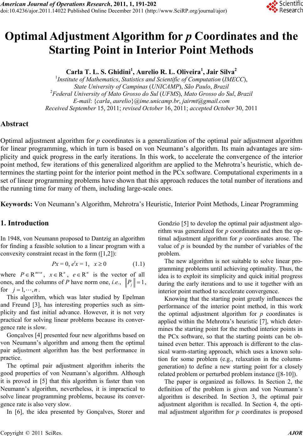
|