American Journal of Oper ations Research, 2011, 1, 220-228
doi:10.4236/ajor.2011.14025 Published Online December 2011 (http://www.SciRP.org/journal/ajor)
Limited Resequencing for Mixed Models
with Multiple Objectives
Patrick R. McMullen
Schools of Business, Wake Forest University, Winston-Salem, USA
Received August 29, 2011; revised September 30, 2011; accepted Oct o b er 12, 2011
Abstract
This research presents a problem relevant to production scheduling for mixed models—production schedules
that contain several unique items, but each unique item may have multiple units that require processing. The
presented research details a variant of this problem where, over multiple processes, re-sequencing is permit-
ted to a small degree so as to exploit efficiencies with the intent of optimizing the objectives of required set-
ups and parts usage rate via an efficient frontier. The problem is combinatorial in nature. Enumeration is
used on a variety of test problems from the literature, and a search heuristic is used to compare optimal solu-
tions with heuristic based solutions. Experimentation shows that the heuristic solutions approach optimality,
but with opportunities for improvement.
Keywords: Sequencing, Heuristics, Simulated Annealing
1. Introduction
Sequencing has been a popular topic in production re-
search for as long as production research has been in
existence. Typically, sequencing is done such that some
objective associated with operational performance is
optimized. Typically, these objectives involve entities
such as labor use, in-process inventories, and flexibility.
1.1. Setups and Usage Rate
Of interest here are two objectives: one objective is con-
cerned with minimization of setups, the other is con-
cerned with stability of materials usage. The first ob ject-
tive is easily understood, while the second is less under-
stood. The stability of materials usage is a matter of
concern to those involved with lean manufacturing sys-
tems involving multiple quantities of each unique item
requiring processing. Scenarios where items require
processing when there are multiple units of each unique
item are frequently referred to as mixed models. Manu-
facturing systems such as this desire some progression of
each item’s processing in proportion to the demand of
the item of interest. A metric associated with the stability
of materials usage was contributed by the seminal work
of Miltenburg [1]. Miltenburg also contributed algo-
rithms concerned with ob taining production sequences to
minimize the material usage rate. To illu strate the princi-
ple of mixed model sequencing, consider a simple exam-
ple where it is required to process four units of item A,
two units of item B and one unit of item C. One possible
sequence is as follows:
AAAABBC (S1)
The sequence above does not accomplish the objective
of stabilizing material usage. All of the As are process,
followed by the Bs, finishing with the Cs. The Milten-
burg metric is optimized when the items are scrambled
such that the presence of each item’s sequence positions
is proportional to its demand. The following sequence
is more desirable with the material usage rate is consid-
ered:
ABACABA (S
2)
In layman’s terms, one may better understand the need
for stabilizing the material usage rate with a variant to
this example. Imagine a scenario where demand is am-
plified by a factor of 1000 and that units A, B and C are
needed by a customer for assembly (1000 assemblies
required). Each single assembly requires four of A, two
of B and one of C. One option is to employ a form of S1
above—producing 4000 of A, then 2000 of B and fi-
nally 1000 of C—a production sequence of 7000 mem-
bers. Now imagine a disaster (a power outage, for exam-
ple) halfway through the sequence—only 3500 units of

P. R. MCMULLEN 221
A were produced. This disaster leaves the customer un-
able to assemble any of the 1000 demanded units—a
death blow to the intentions of JIT/lean systems. On the
other hand, consider employing S2 1000 times and the
same disaster occurs halfway through the sequence.
When S2 is employed, the customer is still able to com-
plete 3500 assemblies, which are 3500 assemblies more
than when the S1 approach is employed.
While S2 has its advantages over S1 in terms of stabil-
ity of material usage, it also has a major drawback—it
results in many setups, frequently changing over from
one unique item to another. S1 is superior to S2 in terms
of setups. In fact, the two objectives of concern here are
in conflict with each other—they are inversely correlated
[2,3]. This is a common affliction for those interested in
multiple-objective optimization [4]. Given the tradeoff
between the number of setups and the stability of mate-
rial usage, there is motivation to find sequences that pro-
vide desirability in terms of both objectives. In fact,
multi-objective optimization problems are rife with con-
flicting objectives [5].
1.2. Sequencing and Limited Re-Sequencing
When multiple processes are required for a production
problem, one can conceivably consider the situation an
opportunity for improving the schedule from process to
process. This “improving” the schedule can come in the
form of re-sequencing. In this context, re-sequencing
suggests making adjustments to the sequence prior to
each process. In reality, these adjustments would typi-
cally be minor in nature, as physical limitations would
prevent any re-sequencing to a large degree. As such, the
re-sequencing associated with this research effort is con-
sidered limited re-sequencing. The work of Lahmar and
Benjaafar [6] describes how physical buffers dictate the
degree of re-sequencing that is feasible. Their work pre-
sents techniques to find desirable sequences, and is ap-
plied to automotive industry applications.
As stated by Lahmar and Benjaafar [6], physical space
availability dictates buffering ability, and subsequently
the degree of re-sequencing that is feasible. For this re-
search effort, it will be assumed that there is buffer space
available to permit re-sequencing of only one item in the
sequence. This means that one item is permitted to be
taken out of the sequence and reinserted into a later part
of the sequence. Figure 1 provides a numerical example
of a feasible re-sequencing:
Here, item A, the first item in the sequence, is taken
AABB |CC (Initial Sequence)
ABBACC (New Sequence)
Figure 1. A feasible re-sequencing.
out of sequence, and later re-inserted. It is pushed back
in the sequence. Meanwhile, the intervening items in the
sequence move forward one position because of item A
being pushed back. Figure 2 shows another type of fea-
sible sequence:
Here, item A is pushed back, as is item B. Despite
multiple pushbacks, this scenario is still feasible, as the
buffer space of one unit is never exceeded. Furthermore,
notice that none of the items have moved up more than
one position in the sequence. Figure 3 shows an illu stra-
tion of an infeasible re-sequencing:
This particular sequence is not permitted. The reason
for this is because the buffer capacity of one unit would
be exceeded. The first two items in the sequence would
be held in buffer at the same time, which is not permitted.
Another indication as to the infeasibility of th is sequence
is that the first item C would have move forward two
positions in the sequence, which is not permitted, given it
exceeds the buffer size of one.
1.3. Multiple Processes and Combinatorial
Difficulties
For some number of processes, limited re-sequencing
can be performed. For three processes, for example, there
are three opportunities for re-sequencing. For each proc-
ess, there is some number of re-sequencing possibilities.
This number of re-sequencing possibilities is equal to the
number of feasible re-sequencing possibilities associated
with the original sequence. In this context, the original
sequence is referred to as the parent sequence, and the
re-sequenced sequence is referred to as the child se-
quence. For example, consider a scenario where two
units of A are demanded, one unit of both B and C are
demanded. From this demand pattern, the trivial se-
quence of AABC is constructed. AABC is considered the
parent sequence for this example. This parent sequence
has 4P2,1,1 = twelve feasible permutations, or sequences.
Of these twelve permutations, there are only four which
are considered feasible in terms of the limited re-se-
quencing with a buffer size of one unit. These sequences
are AABC, AACB, ABAC, and ABCA. In the context of
the description above, these can be considered child se-
quences. Note that the AABC sequence is essentially a
direct mapping of its parent sequence. For the next
AAB|BC|C (Initial Sequence)
ABACBC (New Sequence)
Figure 2. A feasible re-sequencing w ith two pushbacks.
ABC|AAB|BC (Initial Sequence)
CAABBC (New Sequence)
Figure 3. An infeasible re-sequencing.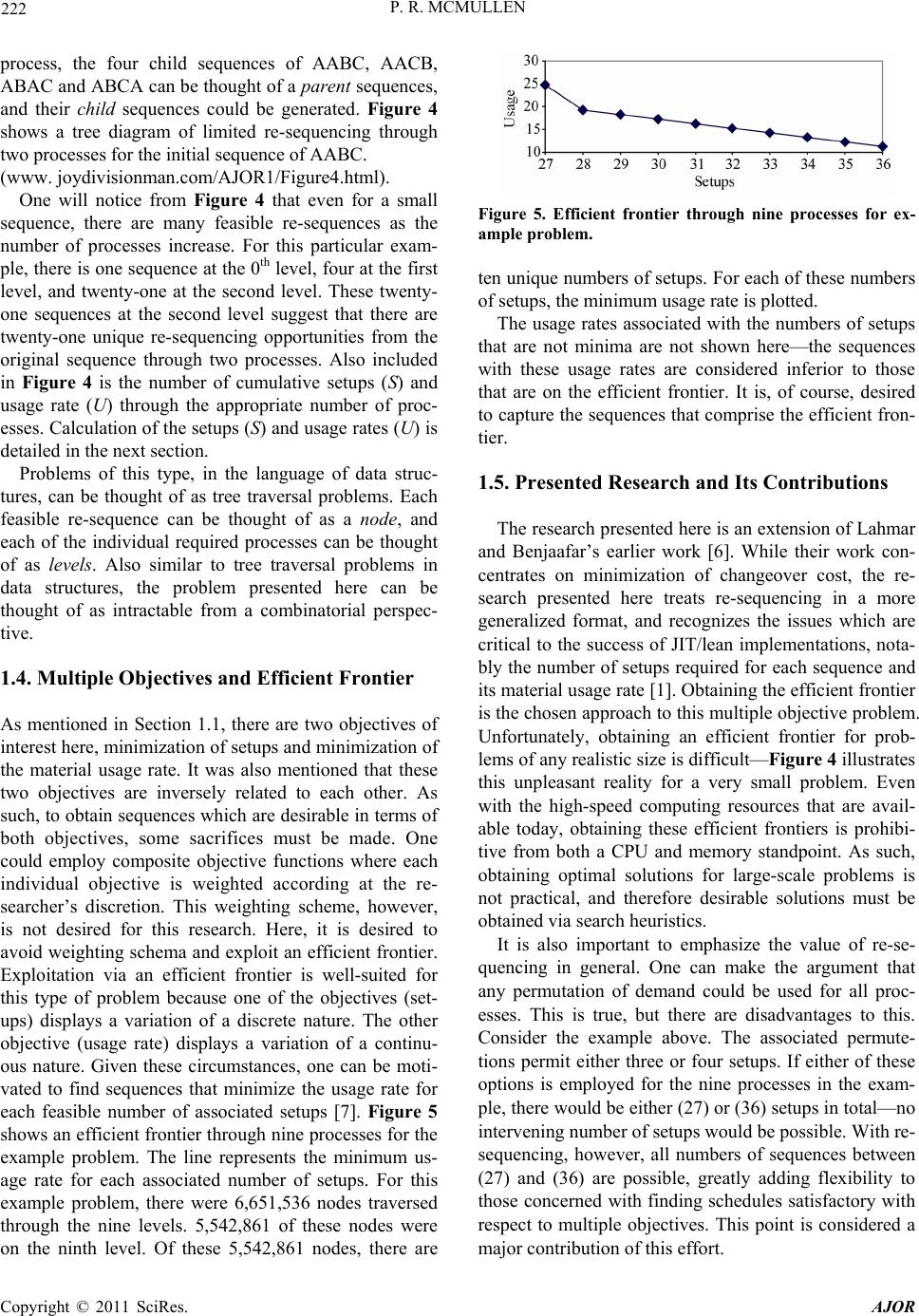

P. R. MCMULLEN
222
process, the four child sequences of AABC, AACB,
ABAC and ABCA can be thought of a parent sequences,
and their child sequences could be generated. Figure 4
shows a tree diagram of limited re-sequencing through
two processes for the initial sequence of AABC.
(www. joydivisionman.com/AJOR1/Figure4.html).
One will notice from Figure 4 that even for a small
sequence, there are many feasible re-sequences as the
number of processes increase. For this particular exam-
ple, there is one sequence at the 0th level, four at the first
level, and twenty-one at the second level. These twenty-
one sequences at the second level suggest that there are
twenty-one unique re-sequencing opportunities from the
original sequence through two processes. Also included
in Figure 4 is the number of cumulative setups (S) and
usage rate (U) through the appropriate number of proc-
esses. Calculation of the setups (S) and usage rates (U) is
detailed in the next section.
Problems of this type, in the language of data struc-
tures, can be thought of as tree traversal problems. Each
feasible re-sequence can be thought of as a node, and
each of the individual required processes can be thought
of as levels. Also similar to tree traversal problems in
data structures, the problem presented here can be
thought of as intractable from a combinatorial perspec-
tive.
1.4. Multiple Objectives and Efficient Frontier
As mentioned in Section 1.1, there are two objectives of
interest here, minimization of setups and minimization of
the material usage rate. It was also mentioned that these
two objectives are inversely related to each other. As
such, to obtain sequences which are desirable in terms of
both objectives, some sacrifices must be made. One
could employ composite objective functions where each
individual objective is weighted according at the re-
searcher’s discretion. This weighting scheme, however,
is not desired for this research. Here, it is desired to
avoid weighting schema and exploit an efficient frontier.
Exploitation via an efficient frontier is well-suited for
this type of problem because one of the objectives (set-
ups) displays a variation of a discrete nature. The other
objective (usage rate) displays a variation of a continu-
ous nature. Given these circumstances, one can be moti-
vated to find sequences that minimize the usage rate for
each feasible number of associated setups [7]. Figure 5
shows an efficien t frontier through nine processes for the
example problem. The line represents the minimum us-
age rate for each associated number of setups. For this
example problem, there were 6,651,536 nodes traversed
through the nine levels. 5,542,861 of these nodes were
on the ninth level. Of these 5,542,861 nodes, there are
Figure 5. Efficient frontier through nine processes for ex-
ample problem.
ten unique numbers of setups. For each of these numbers
of setups, the minimum usage rate is plotted.
The usage rates associated with the numbers of setups
that are not minima are not shown here—the sequences
with these usage rates are considered inferior to those
that are on the efficient frontier. It is, of course, desired
to capture the sequences that comprise the efficient fron-
tier.
1.5. Presented Research and Its Contributions
The research presented here is an extension of Lahmar
and Benjaafar’s earlier work [6]. While their work con-
centrates on minimization of changeover cost, the re-
search presented here treats re-sequencing in a more
generalized format, and recognizes the issues which are
critical to the success of JIT/lean implementations, nota-
bly the number of setups required for each sequence and
its material usage rate [1]. Obtainin g the efficient frontier
is the chosen ap proach to th is multiple obj ective prob lem.
Unfortunately, obtaining an efficient frontier for prob-
lems of any realistic size is difficult—Figure 4 illustrates
this unpleasant reality for a very small problem. Even
with the high-speed computing resources that are avail-
able today, obtaining these efficient frontiers is prohibi-
tive from both a CPU and memory standpoint. As such,
obtaining optimal solutions for large-scale problems is
not practical, and therefore desirable solutions must be
obtained via search heuristics.
It is also important to emphasize the value of re-se-
quencing in general. One can make the argument that
any permutation of demand could be used for all proc-
esses. This is true, but there are disadvantages to this.
Consider the example above. The associated permute-
tions permit either three or four setups. If either of these
options is employed for the nine processes in the exam-
ple, there would be either (27) or (36) setups in total—no
intervening number of setups would be possible. With re-
sequencing, however, all numbers of sequences between
(27) and (36) are possible, greatly adding flexibility to
those concerned with finding schedules satisfactory with
respect to multiple objectives. This point is considered a
major contribution of this effort.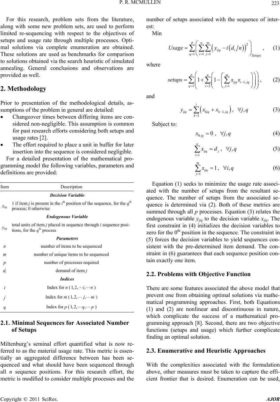

P. R. MCMULLEN 223
For this research, problem sets from the literature,
along with some new problem sets, are used to perform
limited re-sequencing with respect to the objectives of
setups and usage rate through multiple processes. Opti-
mal solutions via complete enumeration are obtained.
These solutions are used as benchmarks for comparison
to solutions obtained via the search heuristic of simulated
annealing. General conclusions and observations are
provided as well.
2. Methodology
Prior to presentation of the methodological details, as-
sumptions of the problem in general are detailed:
 Changeover times between differing items are con-
sidered non-negligible. This assumption is common
for past research efforts considering both setups and
usage rates [2].
 The effort required to place a unit in buffer for later
insertion into the sequence is consid ered negligible.
For a detailed presentation of the mathematical pro-
gramming model the following variables, parameters and
definiti ons are provided:
Item Description
Decision Variable
xijq 1 if item j is present in the ith position of the sequence, for t he qth
process; 0 otherwise
Endogenous Variable
yijq total units of item j placed in sequence through i seque nce posi-
tions, for the qth process
Parameters
n number of items to be sequenced
m number of unique items to be sequenced
p number of processes required
dj demand of item j
Indices
i Index for n (1, ) 2,,in
j Index for m (1) ,2,,jm
q Index for p (1) ,2,,qp
2.1. Minimal Sequences for Associated Number
of Setups
Miltenburg’s seminal effort quantified what is now re-
ferred to as the material usage rate. This metric is essen-
tially an aggregated difference between has been se-
quenced and what should have been sequenced through
all n sequence positions. For this research effort, the
metric is modified to consid er multiple processes and the
number of setups associated with the sequence of inter-
est:
Min
 
2
111
pnm
ijq i
qij Setups
Usageyi dn





 , (1)
where
1,
12 1
11
pnm
ijq ijq
qi j
setupsxx 
 












 
, (2)
and

1,
1
i
ijqkjqk jq
k
yxx





,jq, (3)
Subject to:
00 jq
x

, (4) ,jq
1
n
ijq j
i
x
d


, (5) ,jq
11
m
ijq
j
x


, (6) ,iq
Equation (1) seeks to minimize the usage rate associ-
ated with the number of setups from the resultant se-
quence. The number of setups from the associated se-
quence is determined via (2). Both of these metrics are
summed through all p processes. Equation (3) relates the
endogenous variable yijq to the decision variable xijq. The
first constraint in (4) initializes the decision variables to
zero for the 0th position in the sequence. The constraint in
(5) forces the decision variables to yield sequences con-
sistent with the pre-determined item demand. The con-
straint in (6) guarantees that each sequence position con-
tain exactly one item.
2.2. Problems with Objective Function
There are some features associated the above model that
prevent one from obtaining optimal solutions via mathe-
matical programming approaches. First, both Equations
(1) and (2) are nonlinear and discontinuous in nature,
which complicate the success of a mathematical pro-
gramming approach [8]. Second, there are two objective
functions (setups and usage) which further complicate
finding an optimal solution.
2.3. Enumerative and Heuristic Approaches
With the complexities associated with the formulation
above, other measures must be taken to capture the effi-
cient frontier that is desired. Enumeration can be used,

P. R. MCMULLEN
224
similar to that shown in Figure 4. Unfortunately, enu-
meration is not computationally feasible for large prob-
lems from both a CPU and memory standpoint—prob-
lems of this type are rigorous from a combinatorial
standpoint to a very large degree. For small problems,
enumeration is effective in capturing the optimal effi-
cient frontier.
For larger problems, search heuristics can be used—
algorithms used to obtain desirable, although not neces-
sarily optimal solutions with a reasonable degree of
computational effort. There are many search heuristics
available to the research, but simulated annealing is used
for this particular effort.
2.4. Simulated Annealing Heuristic
Simulated annealing [9,10] is the search heuristic used
for this research. It is acknowledged that there are many
search heuristics available for finding desirable solutions
to combinatorial optimization problems with a reason-
able computational effort. Genetic Algorithms [11], Tabu
Search [12] and Ant Colony Optimization [13] are just a
few. Choosing the “b est” search heuristic for this type of
problem is beyond the scope of the paper, and this point
is emphasized later as an opportunity for subsequent re-
search. The following subsections detail the steps associ-
ated with the search heuristic for the problem of interest.
2.4.1. Initi al i zation (Step 0)
The first step in the heuristic is to initialize all of the pa-
rameters to appropriate values. The relevant parameters
are shown below:
Parameter Description
T1 Initial temperature
TF Final temperature
T Current temperature
Iter Iterations for each temperature level
CR Cooling rate
kB Boltzman constant
Relevant variable values which are endogenous (de-
termined by the search heuristic) are defined as follows:
Variable Description
UsageT[Setups] Usage for test solution with Setups
UsageC[Setups] Usage for current solution with Setups
UsageB[Setups] Usage fo r b e st s o lu t i on w it h Setups
 Relative inferiority of test solution
PA Probability of accepting inferior s ol u tion
An initial sequence is chosen. For this research, the
“trivial” sequence is always used for initialization. The
“trivial” sequence assumes that all item A units will be
placed at the beginning of the sequence, all item B units
are next, etc. The value of the q index is set to zero. Us-
ageC[Setups] and UsageB[Setups] are initialized to very
high values for all possible values of Setups. T is initial-
ized to T1.
2.4.2. Modi fi cation (Step 1)
Modification is performed in a fashion identical to that
shown in Figure 1. Single “pushbacks” are used for the
presented heuristic. The targeted item and its new
“pushback” location are both chosen randomly according
to a uniform probability distribution. The resultant se-
quence in process q is the parent sequence for process q
+ 1. In the spirit of the example problem shown in Fig-
ure 4, here’s an example of modification through four
processes.
Process: q = 0 q = 1 q = 2 q = 3 q = 4
Seq. AABCABACABCA BACABAAC
Note how that for each subsequent process, an item
never moves forward more than one position in the se-
quence—this is the enforcement of the constraint re-
stricting the buffer size to one.
2.4.3. Ob jective Function ( Step 2 )
After modification is performed for all p processes, the
number of Setups and Usage rates are determined ac-
cording to Equations (1) and (2). Continuing with the
example above, Setups and Usage values through each of
the four processes are as follows:
Proc.(q): 0 1 2 3 4
Seq: AABC ABAC ABCA BACA BAAC
S/U: N/A 4/1.75 4/1.25 4/1.75 3/2.25
S/UN/A 4/1.75 8/3.00 12/4.75
15/7.00
The most important values associated with these p
modifications are the cumulative Setups and Usage val-
ues for the pth process. This is considered the objective
function value. For this example, the four modifications
resulted in a Usage rate of 15.00 for the (15) associated
Setups. Again, it is desired to minimize the Usage rate
for each associated number of Setups. This usage rate is
referred to as UsageT[Setups].
2.4.4. Comp arison (Step 3)
The desirability of the objective function is compared to
that of the current solution via their Usage rates associ-
ated with their Setups. If th e Usage rate for the test solu-
tion is less than that of the current solution, the test solu-

P. R. MCMULLEN 225
tion replaces the current solution. If the Usage rate for
the test solution is less than that of the best solution, the
test solution replaces the best solution.
Otherwise, the Metropolis criterion for replacing a
current solution with one having relative inferiority is
explored [8,9,14]. The relative inferiority of the test so-
lution is computed via the following:





TC
C
Usage SetupsUsageSetups
Usage Setups


 (7)
The probability of accepting this relatively inferior
solution is determined as follows:

exp
A
Pk  

B
T (8)
A random number on the (0, 1) interval is generated
according to a uniform distribution. If this value is less
than PA, the relatively inferior test solution replaces the
current solution. Otherwise, the current solution remains
current.
2.4.5. Incrementation (Step 4)
Steps 1 through 3 are repeated Iter times. After Iter times,
the current temperature is adjusted according to the fol-
lowing relation:
TTCR (9)
This pattern continues while T exceeds TF.
2.4.6. Completion (Step 5)
When the value of T no longer exceeds TF, the search
heuristic stops, and the efficient frontier values (UsageB
[Setups]) are reported.
2.4.7. Pseud ocode
The steps below show the steps of this heuristic in pseu-
docode:
3. Experimentation
To measure the performance of the heuristic methodol-
ogy presented, several test problems are used to compare
optimal solutions via enumeration to those found via the
heuristic. Some of these test problems are from the lit-
erature [15]; some are new with this research. These
problem sets are listed in the Appendix.
3.1. Performance Measures
The overall measure of performance is essentially two-
fold. The first measure of performance is classified as
relative inferiority—the degree to which the efficient
frontier associated with the heuristic search is above, or
inferior to, the efficient frontier obtained via enumeration.
The second performance measure is the number of fron-
tier voids—the frequency of the efficient frontier (ob-
tained via the heuristic) not providing a specific solution
yielding a number of setups yielded by the optimal solu-
tion (obtained via enumeration). It is, of course, desired
that the relative inferiority and the number of frontier
voids both be minimized.
Figure 6, an extension of Figure 5, shows an example
of the original efficient frontier, alongside a hypothetical
efficient frontier obtained via the simulated annealing
heuristic.
From this illustration, one will note that the efficient
frontier obtained via the heuristic can only equal, never
surpass, the optimal heuristic obtained via enumeration.
The relative inferiority of the efficient frontier obtained
via the heuristic approach is the average degree to which
it is above the optimal frontier. The value of this per-
formance measure is straightforward when the following
notation is used:
Notation Definition
UsageOptimal[Setups]Us a g e r a t e for o p t i mal solution with Setups
UsageSA[Setups] Usage rate for heursitc solution with Setups
MinS Minimum number of setups
MaxS Maximum number of setups
Initialize();
while(T > TF){
for(h = 1; h <= Iter; h++){
modification();
determineObjectiveFunction();
if(UsageT[Setups] < UsageC[Setups]){
replaceCurrent();
if(UsageT[Setups] < UsageB[Setups])
replaceBest();}
else testMetropolisCriterion();}
T = T*CR;}
reportEfficientFrontier();
The relative inferiority of the heuristic solution can
then be determined via the following:

 

max
min
1
..
1max min
SSAOpt
iS Opt
Rel InfSS
Usagei Usagei
Usage i




(10)
For this example, the relative inferiority of the heuris-
tic solution is 4.90%.
To illustrate the concept of frontier voids, another
variant of Figure 5 is presented via another hypothetical
heuristic solution to the original problem shown in Fig-
ure 7.

P. R. MCMULLEN
226
Figure 6. Efficient frontiers obtained via enumeration and search heuristic.
Figure 7. Example of one frontier void.
For this example, there is one frontier void—the heu-
ristic did not find a solution associated with (34) setups.
The relative inferiority associated with this solution is
calculated the same way as described above, except that
the frontier void statistics are omitted from the calcula-
tion, resulting in a denominator decrease equal to the
number of frontier voids—in this case (34) Setups and
the Usage rate of 13.25, resulting in a relative inferiority
of 4.82%.
frontier so that a comparison can be made to optimal.
The parameters used for the simulated annealing search
are adjusted according to problem size, so that the search
is proportional to the number of nodes encountered via
enumeration.
3.3. Computational Experience
The capturing of the optimal efficient frontier via both
enumeration and simulated annealing was done via pro-
grams written with the Java Development Kit, version
1.6.02 and executed on the Microsoft Vista operating
system with an AMD Turion 64 × 2 processor. CPU
times for the enumeration effort are reported in the re-
sults section. CPU times for the simulated annealing
heuristic effort were not of consequence and are not re-
ported. The number of nodes associated with the enu-
merative search is reported in the results section, as this
measure discloses how much memory is required for the
traversal of the search tree.
3.2. Problem Size
As stated earlier, the problem sets used are detailed in the
Appendix. For each unique problem, multiple processes
are explored, from as few as p = 2 to as large as p = 10.
From Figure 4, there were only p = 2 processes used.
The more processes used, the more rigorous the search.
Across all problem sets and ranges of processes, there
are (90) total problems studied. Table 1 details the range
of depth used for the various problem sets.
For each of the (90) problems studied, the optimal ef-
ficient frontier is captured via enumeration. The simu-
lated annealing heuristic is then used to find the efficient
It is also noted here that the simulated annealing heu-
ristic parameters of iterations (Iter), cooling rate (CR)
and the Boltzman constant (kB) were determined for each
test problem in a manner propo rtional to the total number
of nodes. Specifically, these three parameters were cho-
sen so that the simulated annealing heuristic search space
was 10% of the size of the total number of nodes.
Table 1. Depth of re-sequencing problems.
Problem Set Range of Processes (p)
A0 p = 2, p = 10
A1 p = 2, p = 4
A2 p = 2, p = 4
A3 p = 2, p = 4
A4 p = 2, p = 6
A5 p = 2, p = 9
4. Experimental Results
Tables 2(a)-(f) (http://www.joydivisionman.com/AJOR1/
Table2.html) show the performance results of the six

P. R. MCMULLEN 227
problem sets used for this research. Nodes is the number
of sequences encountered in the enumerative search tree.
CPU Time (in minutes) the length of time the CPU spent
finding the optimal solution via enumeration. Inferiority
is the degree to which the heuristic was inferior to the
optimal solution. Voids depicts the number of times that
the heuristic search failed to find a solution correspond-
ing with the number of setups for the optimal solution.
4.1. Results for Problem Sets
Tables 2(a)-(f) are available on the internet via
www.joy-divisionman.com/AJOR1/Table2.html.
4.2. Interpretation of Results
For the (90) problems studied, the simulated annealing
heuristic provided a solution that was, on average, 3.74%
above (or inferior to) the optimal solution obtained via
enumeration. The sum of the frontier voids across all (90)
problems as compared to the total number of unique set-
ups across all problems is 9.48%.
The CPU time required to solve the problems to opti-
mality illustrates a few forces at work. One force is the
number of processes involved in the enumeration (p). As
p increases, the number of nodes increases to an expo-
nential degree. Another force at work is the number of
permutations associated with each individual problem.
As the number of permutations associated with the prob-
lem increases, the number of potentially feasible child
sequences also increases, and these must potentially fea-
sible sequences must be examined for feasibility. The
number of items in the sequence (n), and the number of
unique items in the sequence (m) also dictate computa-
tional resource needs. Of course, as n and m increase, so
does the number of permutations that must be checked
for feasibility.
5. Research in Perspective
This research was mainly dedicated to presenting a prob-
lem and associated solution which can be used to en-
hance the competitive positions of organizations con-
cerned with multiple-objective sequencing over several
processes. While the author considers an average inferi-
ority of 3.74% to optimal reasonable, frontier voids of
9.48% is considered a performance where improvement
is desired. The following sections detail further research
limitations, as well as suggestions for subsequent oppor-
tunities.
5.1. Limitations of Research
There are a few limitations to this research which should
be itemized. First of all, as mentioned earlier in the paper,
the buffer size is one unit throughout. This means that
only one item can be withheld and later reinserted into
the sequence, which ultimately means that when re-se-
quencing for a single process, a unit can only move up
one position in the sequence. A buffer size of one does
limit the flexibility of the research.
Another limitation of this research is an assumption
that cannot be avoided in one form or other—the initial
sequence used. For purposes of consistency, the initial
sequence (the level 0 sequence) used for this effort was
always one where the item A’s were sequenced first,
followed by the item Bs, and so on. Re-sequencing was
then performed. The result of this assumption was that
the efficient frontiers were always well-represented on
the low-setup end, but the high-setup end of the efficient
frontier was frequently the source of inferiority and/or
frontier voids. Nevertheless, this initial sequence as-
sumption was made in the interest of consistency. Other
assumptions could be considered for initial sequences,
but this is left as a future research opportunity.
Another limitation associated with this research is as-
sociated with the problem size. Despite some of the
enumerated solutions showing more than 20 million
nodes, the problems used for experimentation could be
considered, from a combinatorial sense, small. Of course,
finding solutions via the simulated annealing heuristic
has no real size limitations, but the optimal solutions
obtained via enumeration provide a basis for comparison.
Given this, simulated annealing was only done for prob-
lems that could be solved via enumeration as well. The
constraining factor for finding optimal solutions for this
research had more to do with system memory than the
CPU. This caveat is not uncommon for problems requir-
ing tree-traversal [16].
5.2. Opportunities for Future Research
Fortunately, some of the limitations associated with this
effort also provide opportunities for new research efforts.
One obvious opportunity is to improve the performance
of the heuristic approach, especially regarding frontier
voids. This could be explored via other search heuristics,
such as tabu search, genetic algorithms, or natural agent
systems such as ant-colony optimization.
Another opportunity for further research relates to the
number of buffers used. For this research, a buffer-size
of one was used throughout. This restricts re-sequences
to be limited to moving up no more than one unit. Larger
buffer sizes would permit more flexibility in re-se-
quencing in this regard. On the down side of this, how-
ever, more computational recourses are needed for larger
buffer sizes, in terms of both CPU and memory resources.

P. R. MCMULLEN
228
With computing resources in a state of perpetual growth,
larger buffer-sizes are not unrealistic in the future.
The size of the problems studied is also something that
could be further explored as computing resources be-
come more plentiful. At present, some of the smaller
problem sets of earlier research were used [15]. Some
larger problem sets from this research could be used as
computing resources permit. The problem sets can be
found via
www.joydivisionman.com/AJOR1/Appendix. html.
6. References
[1] J. Miltenburg, “Level Schedules for Mixed-Model As-
sembly Lines in Just in Time Production Systems,” Man-
agement Science, Vol. 35, No. 2, 1989, pp. 192-207.
doi:10.1287/mnsc.35.2.192
[2] P. R. McMullen, “JIT Sequencing for Mixed-Model As-
sembly Lines Using Tabu Search,” Production Planning
and Control, Vol. 9, No. 5, 1998, pp. 504-510.
doi:10.1080/095372898233984
[3] P. R. McMullen and G. V. Frazier, “A Simulated An-
nealing Approach to Mixed-Model Sequencing with Mul-
tiple Objectives on a Just in Time Line,” IIE Transaction s,
Vol. 32, No. 8, 2000, pp. 679-686.
doi:10.1080/07408170008967426
[4] A. Joly and Y. Frein, “Heuristics for an Industrial Car
Sequencing Problem Considering Paint and Assembly
Shope Objectives,” Computers & Industrial Engineering,
Vol. 55, No. 2, 2008, pp. 295-310.
doi:10.1016/j.cie.2007.12.014
[5] M. Masin and Y. Bukchin, “Diversity Maximization Ap-
proach for Multiobjective Optimization,” Operations Re-
search, Vol. 56, No. 2, 2008, pp. 411-424.
doi:10.1287/opre.1070.0413
[6] M. Lahmar and S. Banjaafar, “Sequencing with Limited
Flexibility,” IIE Transactions, Vol. 39, No. 10, 2007, pp.
937-955. doi:10.1080/07408170701416665
[7] P. R. McMullen, “A Kohonen Self-Organizing Map Ap-
proach to Addressing a Multiple Objective, Mixed Model
JIT Sequencing Problem,” International Journal of Pro-
duction Economics, Vol. 72, No. 1, 2001, pp. 59-71.
doi:10.1016/S0925-5273(00)00091-8
[8] LI N GO, “The Mo deling Language an d Optimizer,” LINDO
Systems, Inc., Chicago, 1995.
[9] S. Kirkpatrick, C. D. Gelatt and M. P. Vecchi, “Optimi-
zation by Simulated Annealing,” Science, Vol. 220, No.
4598, 1983, pp. 671-679.
doi:10.1126/science.220.4598.671
[10] R. W. Eglese, “Simulated Annealing: A Tool for Opera-
tional Research,” European Journal of Operational Re-
search, Vol. 46, No. 3, 1990, pp. 271-281.
doi:10.1016/0377-2217(90)90001-R
[11] J. H. Holland, “Adaptation in Natural and Artificial Sys-
tems,” University of Michigan Press, Ann Arbor, 1975.
[12] F. Glover, “Tabu Search: A Tutorial,” Interfaces, Vol. 20,
No. 1, 1990, pp. 74-94. doi:10.1287/inte.20.4.74
[13] M. Dorigo and L. M. Gambardella, “Ant Colonies for the
Traveling Salesman Problem,” Biosystem, Vol. 43, No. 1,
1997, pp. 73-81. doi:10.1016/S0303-2647(97)01708-5
[14] N. Metropolis, A. Rosenbluth, N. Rosenbluth, A. Teller
and E. Teller, “Equation of State Calculations by Fast
Computing Machines,” Journal of Chemical Physics, Vol.
51, No. 6, 1953, pp. 177-190.
[15] P. R. McMullen, “An Ant Colony Optimization Ap-
proach to Addressing a JIT Sequencing Problem with
Multiple Objective,” Artificial Intelligence in Engineer-
ing, Vol. 15, No. 3, 2001, pp. 309-317.
doi:10.1016/S0954-1810(01)00004-8
[16] R. Sedgewick, “Algorithms in Java,” 3rd Edition, Addi-
son-Wesley, New York.