American Journal of Oper ations Research, 2011, 1, 293-304
doi:10.4236/ajor.2011.14034 Published Online December 2011 (http://www.SciRP.org/journal/ajor)
293
Average Power Function of Noise and Its Applications in
Seasonal Time Series Modeling and Forecasting
Qiang Song
RedPrairie Corporation, Alpharetta, USA
Received August 29, 2011; revised Septembe r 25, 2011; accepted Octo ber 11, 2011
Abstract
This paper presents a new method of detecting multi-periodicities in a seasonal time series. Conventional
methods such as the average power spectrum or the autocorrelation function plot have been used in detecting
multiple periodicities. However, there are numerous cases where those methods either fail, or lead to incor-
rectly detected periods. This, in turn in applications, produces improper models and results in larger fore-
casting errors. There is a strong need for a new approach to detecting multi-periodicities. This paper tends to
fill this gap by proposing a new method which relies on a mathematical instrument, called the Average
Power Function of Noise (APFN) of a time series. APFN has a prominent property that it has a strict local
minimum at each period of the time series. This characteristic helps one in detecting periods in time series.
Unlike the power spectrum method where it is assumed that the time series is composed of sinusoidal func-
tions of different frequencies, in APFN it is assumed that the time series is periodic, the unique and a much
weaker assumption. Therefore, this new instrument is expected to be more powerful in multi-periodicity de-
tection than both the autocorrelation function plot and the average power spectrum. Properties of APFN and
applications of the new method in periodicity detection and in forecasting are presented.
Keywords: Seasonal Time Series, Forecasting, Seasonality Detection, Average Power Function of Noise,
Average Power Spectrum, Autocorrelation Functions
1. Introduction
Recently, modeling and forecasting seasonal time series
with multiple periodicities has regained attentions from
researchers [1-8]. There is an abundance of literature on
modeling and forecasting time series with a single period
[9,10]. However, with multiple periodicities existing in a
seasonal time series, modeling and forecasting such a
time series becomes quite complicated. An important
task in modeling su ch time series is the determination of
the cycle length of each period. In the literature of mod-
eling and forecasting seasonal time series with multi-
periodicities, the lengths of periods are determined by
human beings, based on either their experience or their
specific domain knowledge of the time series under
study. For example, in determining the cycle lengths of
periods in modeling and forecasting daily electricity load
[7] two distinct periods are determined manually based
on power spectrum and autocorrelation plots, one being
the intraday period which corresponds to 24 hours, and
the other being the intraweek period which corresponds
to 168 hours. When the plurality of time series to work
with is small, it may not be a significant problem for
human beings to determine the length of each period.
Nevertheless, it will become a forbidding task if the
number of time series is in the range of tens of thousand s,
not to mention the possibility that the periodicities may
change over time. In this case, one has to resort to auto-
mated algorithms to detect the periodicities in a time
series.
Traditionally, the average power spectrum and the
autocorrelation functions have been used in detecting
multiple periods [9-11]. Usually, if the number of peri-
ods M in a seasonal time series is pre-determined, then
the periods corresponding to the largest N peaks of the
average power spectrum will be the periods in the time
series [11, p. 161]. With ACF plot, one looks at the re-
peating peaks and decides proper periods [9, p. 342].
However, there is a certain degree of subjectivity with
those two approaches. This is reflected in applications

Q. SONG
294
where not all the M largest peaks of the average power
spectrum are used in estimating the periods and not all
the repeating peaks on the ACF plot are used as the pe-
riods [5], and there could be conflicting outcomes from
those two approaches. For instance in [5], two periods,
224 and 32, are determined for the five Central Teleph-
ony series. Period 224 corresponds to the l arge st peak on
the power spectrum plot while the peak at lag 224 on the
ACF plot is even not significant at the confidence level
of 0.95. Period 32 corresponds to a very small and even
ignorable peak on the power spectrum; however, it con-
curs with a significant peak (at the confid ence level 0.95)
at lag 32 on the ACF plot (see Figure 4 and Figure 5 of
[5] for details). It couldn’t be an easy job to manually
choose 224 and 32 as the periods before actually running
the forecast. This apparent contradiction lies in the sub-
jectivity in detecting periods using the average power
spectrum and the ACF plots, and for this reason it re-
quires human intervention, modeling experience, and
even domain knowledge.
For the past decades, the average power spectrum has
been utilized as a powerful apparatus in analyzing the
distribution of the energy of a signal over different fre-
quencies. It helps detect frequency components in a sig-
nal. Undoubtedly, this tool is extremely helpful in signal
analysis, communications, circuitry design, and many
other areas. Nevertheless, the average power spectrum
may not be as effective as one would expect in deter-
mining periods in seasonal time series and forecasting
simply because the frequencies or the periods with the
strongest energy may not be the right periods needed in
forecasting. Figure 11 in this paper presents a time series
of the daily sales at a retail store for over one year period
of time. This time series exhibits 3 major different peri-
ods: 7, 28 and 364 due to the operational business cycles.
On the sample ACF plot in Figure 12, there are signifi-
cant peaks at lag 7 and at lag 28, and both are significant
at the significance level of 0.95. However, the peak at lag
364 is not significant at the significance level of 0.95. At
lag 28, the ACF plot has the largest peak. At lag 7, the
ACF plot has the second largest peak. On the sample
power spectrum in Figure 13, period 7 has the largest
peak, and period 31 has the second largest peak. Now, let
us suppose we need to determine the periods of this time
series, and we pick the highest peaks on either the ACF
plot or the power spectrum which is common practice in
the literature. Here is the dilemma with the power spec-
trum and the ACF methods: If only two periods are cho-
sen, those two methods would generate different results.
Seasonal time series repeats itself after a certain time
lag [9], in spite that du e to the noise in th e time series the
degree to which the time series repeats varies. The right
period should be the one at which the time series repeats
itself with the smallest discrepancy, not necessarily the
one repeating the most frequently but with a larger dis-
crepancy. The largest peak on the power spectrum is the
period in which the time series repeats the most fre-
quently. For example, in the illustrative time series in
Figure 11, the sample power spectrum has the largest
peak at period 7. This is because the business activity of
the store repeats week after week, and this pattern re-
peats the most frequently. However, the state of the
business of the store in different weeks of the same
month could be quite different due to different patterns
of customer spending behaviors. Thus, it is hard to say
that the business repeats itself v ery well week after week.
Looking at the time series plot, it seems that the business
of the store repeats much better month after month than
week after week. However, the sample power spectrum
does not have the largest peak at period of 28. Instead, it
has a peak at period 31. The sample ACF plot of this
time series has the largest peak at lag 28; but, this is not
consistent with the sample power spectrum. A deadlock
has been encountered here in selecting a period for this
seasonal time series based on the ACF plot and the
power spectrum plot. Therefore, it is necessary to search
for a new and different apparatus that does not depend on
the frequencies in the time series, but depends on the
degree to which the time series repeats itself. The goal of
this paper is to presen t the construction and properties of
such an instrument, namely, Average Power Function of
Noise.
This paper is organized as follows. In Section 2, the
definition and properties of Average Power Function of
Noise are presented. Distribution of the local minimum
of the sample APFN is discussed in Section 3, followed
by a discussion of measure of seasonality in Section 4.
Three illustration examples are presented in Section 5,
and conclusions and discussions are given in Section 6.
2. The Average Power Function of Noise and
Its Properties
In general, a seasonal time series exhibits periodic be-
havior with period p, or a seasonal time series repeats
itself after p basic time units [9, p. 327]. However, due to
the noise in the time series, a seasonal time series rarely
repeats itself in a perfect fashion. There is always dis-
crepancy when comparing the observations of a seasonal
time series at two different times over exactly p time unit
span. Mathematically, a seasonal time series can be de-
scribed as




x
tp xtt

  where


t

is the
discrepancy and p is the period. Here, p should be under-
stood as the minimum integer value that can be found
and is greater than 1. This discrepancy, when processed
properly, could be an indicator of periodicity of the sea-

Q. SONG
295
Definition 1 (Average Power Function of Noise): Let


x
t be a stochastic process. Then, for any given real
numbers

, if the following limit exists, it will be called
the Average Power Function of Noise (APFN) of


x
t
at lag

:
sonal time series. This is because if the time span be-
tween two observations is indeed the period of the sea-
sonal time series, the discrepancy should be smaller than
if the time span is not the period of the seasonal time
series. If the seasonal time series possesses multiple pe-
riods, then the discrepancies at different periods may be
quite different. A smaller discrepancy indicates a closer
and better similarity between the observations at differ-
ent times with zero discrepancy being the perfect and
ideal case. We will explore and extend this idea in this
section.
 

2
APFN limd
2
T
TT
xt xt
Et
T














 (1)
Obviously,


APFN

is an even function of

if


x
t is periodic. First, we consider the case where


x
t has a unique period p. Then, we have the follow-
ing major result.
Without loss of generality, we will work with stochas-
tic processes and extend the obtained results to time se-
ries in the sequel. In literature, discrepancies can be in
various forms, such as absolute deviations, square of
errors, and even absolute relative errors, just to name a
few. Therefore, it is quite likely to obtain certain results
parallel to what will be reported in this paper, if different
forms of discrepancies are adopted. In this paper, we
choose the square of errors as the form of discrepancy
simply because of its good analytical properties.
Theorem 1. Let


x
t be a stochastic process and be
expressed as




x
tat t

 where


at is the
mean process of


x
t, i.e., , and is a
deterministic function of t, and

at
 
t

Ex

t

is a white noise
process, i.e.,


t

follows

2
0,N


. If


at is a
periodic function of t with a unique period p so that




atat p

, then AP

FN


has a strict local
minimum when p


.
Proof: As



 
x
tp atptp 

 , if setting
p


in (1), then (1) can be written as
First, we present the definition of Average Power
Function of Noise, the corn er stone of this paper.
 




22
22
APFNlimd limd
22
2
limd
2
T T
T T
T T
T
TT
at pt pattt pt
pE tE
TT
tptp tt
Et
T
 

 
 


t


 





 



 







Exchanging the order of integration and expectation
above and noticing that

tp 

and

t

are inde-pendent, we obtain
 
22
22
22
APFNlimd limd 2
22
T T
T T
T T
Etp tpt t
pt
TT

t

 

 
 


 










(2)
When

,pNp



 where 0

 and


,Np

is a neighborhood of p, we have
 



       
2 2
2 2
APFNlimd limd
22
2
lim d
2
TT
TT
TT
T
TT
xt pxtat ptpatt
pE tE
TT
atp atatp attpttpt
E t
T


 



t






 

 


 

 
 
 
 



Exchanging the order of in tegration and mean calcula-
tion and noticing that

t

is white noise and




0at pat

 , we will get
That is, we have


APFN APFNp


p. (3)
 

 
22
2
22
2
APFN limd
2
limd22
2
T
TT
T
TT
at pat
pE T
at pat
Et
T

t










  




 










Therefore,


AP FN

has a strict local minimum at p.
This finishes the proof.
One of the forecasting methods, called naïve method,
is to use the most recent history data as the forecast of
the future. Here, if we use the history data exactly

time units ago as the forecast, then



x
tx  t can

Q. SONG
296

be interpreted as the forecasting error of

xt

 using


x
t. Thus, (1) may be interpreted as the average power
of forecasting errors using the naïve method. Theorem 1
implies that if a stochastic process is seasonal and if we
use the right period in the naïve method to predict its
future, the mean square function of the forecasting errors
will have a local minimum. Intuitively, this is quite
natural as for seasonal stochastic process, observations
with the same periodicity are quite close to each other
and therefore the differences are minimal. One of the
merits of (1) is that it relates periods in a seasonal sto-
chastic process to a type of forecasting errors in a natural
way. This gives one an instrument helpful in detecting
periods from multiple candidates: When detecting peri-
ods for a seasonal stochastic process, select those periods
that correspond to the smallest APFN values in (1). Fig-
ure 14 presents the plot of the sample APFN of the sea-
sonal time series of daily sales at a retail store. It can be
seen that the APFN plots have a local minimum at period
7, 28, and 364, and the values of APFN at those three
periods are different.
With Theorem 1, it is easy to prove the follow ing cor-
ollaries which assume that


x
t

has a unique period.
Corollary 1.

APFN

has the same periods as


x
t if x(t) itself is periodic.
Corolla ry 2 . If p is a period of


x
t, then


NAPF

has a strict local minimum at any integral multiples
where n is a nonzero integer. That is, if p is a period of
np


x
t, then the corresponding local minima will repeat
with the same period.
Corollary 3. If


x
t is a white noise, then

APFN

is a constant with respect to

.
Corollary 4. Let APFN* be the global minimal value
of the average power function of noise. Then, we have
*2
2AP FN


, or *2
APFN
2


.
Corollary 4 implies that the global minimal value of
APFN, when divided by 2, can be used as an upper
bound of the variance of the noise in the stochastic proc-
ess. This will be seen very useful in estimating the fore-
casting error variance.
A seasonal stochastic process may have multiple pe-
riods. Now, let us consider the potential sources that
contribute to the error or discrepancy when forecasting a
seasonal stochastic process, including processes with a
unique period and multiple periods. Of course, the major
source is the noise in the data. This noise will always
produce error in forecasting. There is a second source,
however, that is any improper time lags chosen in fore-
casting


xt


when multiple periods exist. For dif-
ferent values of

, the errors could be quite different.
This is reflected in the APFN plot which exhibits multi-
ple local minima with different values. We intend to in-
terpret this phenomenon by means of the conditional
variance of the noise defined as a deterministic periodic
function of

. With this said, we could have the fol-
lowing theorem.
Theorem 2. Let


x
t be a stochastic process and be
expressed as






x
tat t

 where


at is the
mean process of


x
t and is a deterministic periodic
function of t, and


t

is a noise process which follows


2
0,N


and the conditional variance
 

2
 Et t


  is a deterministic periodic


function of

and
 
0
i
Etp t 





. If both


at and



 have the same periods i so that p




i
pat at,



 has a local minimum when
i
p


and




i
p  
j where ,
then there exists a such that 1, 2,,iM

APFN

has a global
minimum when i p


where 1. jM
Proof: Let be one period. It can be shown that
i
p









  
22
22
2
APFN lim
im
iT
T
TT
pE



d
2
2
ld
2
Tii
T
ii
tptp ttt
T
Etptpt t
t
T





 








  





In the above, it is assumed that the orders of the inte-
gration and the expectation operations can be exchanged. Conditioning the expectation on

t

, we obtain
 
 
    
22
2
EE t
E tp2
2
APFN limd
2
2()
lim d
2
Tii
iT
T
Tii
TT
pt pttt
pt
T
EtEtEtptEtt
T

 






 



 
 
 
 
 



As

2
Et t 


function of

and
 
0
i
Etp t 





is a deterministic periodic  

, we have

297 Q. SONG
 

22
APFN limd
2
Ti
iT
T
EEt pt
pt
T












2
i
p




When i p


,
 
      
        
      

  

2 2
2 2
2 2
2
APFN limd
2
2
limd
2
2
limd
2
T
TT
T
TT
T
at atat attttt
Et
T
EEat atat attttttt
T
at at EEat attttEEtttt
T










 



 

 

 

 



 






   


2
limdAPFN
2
T
T
Ti
T i
T
EEt ptttp
T














for in the above
 
2
limd 0
2
T
TT
atat t
T



 
,
 
0Et t   , and



0Et  
Therefore, i is a strict local minimum.
Among the M local minima, there must be one that is the
smallest, and that minimum must correspond to a certain
period

APFN p

j
p. This finishes the proof.
Theorem 2 explains why the APFN could have multi-
ple local minima with different values in the case where
multiple periods exist: it is due to the conditional vari-
ance function of

t

which has different values at
different periods.
From Corollary 2, we can prove that if is a period
of i
p

x
t for , then 1, 2,,iM

AP FN

will have
a local minimum at any multiples of i, i.e.,
i is also a local minimum. Hence, we have
the following con clusion.
p

FN

AP np
Corollary 5. If

x
t
APF has multiple distinct periods
12 , then ,,, m
pp p

N

has a strict local mini-
mum at each period where .
i
From Theorem 2, we may conclude that not all periods
have equal APFN values. The period that yields the
global minimum APFN value is the most important one
and is the one that must be found in modeling as it may
produce the smallest forecasting error using the naïve
method. For this reason, we give the following defini-
tion.
np 1, 2,,iM
Definition 2. Suppose

x
t

is a stochastic process
and can be expressed as

x
tat t

 where

at is a deterministic periodic function of t and


t

is a noise process which follows

2
0,N



and the
conditional variance


()t 
2
Et   is a determinis-
tic periodic function of

. Suppose also that both


at
and



2()Et t
  have the same periods
i
p
where 1, 2,,iM

, then the period that yields the
smallest APFN value is called the primary period while
all others secondary periods.
Hence, if only one period is chosen for a seasonal sto-
chastic process, it should be the primary period. How-
ever, one may not be able to find the primary period if
using the power spectrum or ACF plot.
The APFN plot can also be used to identify if a deter-
ministic trend exists in a process.
Corollary 6. If


x
tbt t

 where is a non-
zero constant andb


t

is a white noise process, then


APFN

is an increasing function of

.
To apply APFN in detecting the cycle lengths of mul-
tiple periods for a seasonal stochastic process, we rec-
ommend the following outline which can be used as a
basis in designing detailed algorithms.
Step 1. Determine the number of periods, M, to be de-
tected for a given seasonal time series;
Step 2. Calculate APFN(t) using formula (4) to be
given in the next section for different integer values of t;
Step 3. Detect all local minima of APFN(t) and find
the corresponding values of t;
Step 4. Sort all the local minima from the least to the
greatest, and rearrange the corresponding t values ac-
cordingly. Then, the t values of the first M local minima
are the cycle lengths, and the first t value is the primary
period.
Some comments are in order regarding the number of
data points required in calculating the value of APFN(t).
In applications, one uses the sample APFN function in
detecting cycle lengths. Evidently, the more data used in
calculation, the more reliable the results. Although it is
not clear at this stage what the minimum number of data
points should be needed in calculating APFN, our em-

Q. SONG
298
pirical results suggest that it is reasonable to have at least
50 data points in calculating each value of APFN in or-
der to get good results. Nevertheless, this is still an op en
problem that requires more research.
3. Distribution of Local Mini ma of the
Sample Average Power Functions of Noise
In applications and especially when working with time
series, we use the following form of definition of APFN:
 

2
1
1
APFN limN
Nt
pxtp
N
 

xt (4)
As local minima of the APFN are the only interest to
us, and at each local minimum




at pat , denote






pttp
  t . Then, the above Equation (4)
can be written as
 
2
1
1
APFN limN
Np
t
pt
N

 
.
Now, we want to derive the distribution of APFN(p)
for any finite values of N. As

t

follows


2
0,N


by assumption, we know that






pttp
  t
follows


2
0,2N


. Furthermore, we can infer that


pt
 is independent of p where

t  

m0m

, and


2
pt
 follows


1
2
 . It is easy to see that




22
2
p
Et


 . To find the variance of


2t

p, notice
that






22 0ttpcov ,


,








0tp 
2
cov ,tt 

, and








t tp 
2
cov ,tp  0

. Then, we would have,














 

22 2
22
var var2
varvar4var
pttpttpt
tptt tp



 
As














2
24 2
44
44 2
42
var
as 0
3as () follows 0,
2var.
tEt Et
Et Et
tN
tp




 
 




 

 





 


 
 


 






 
2
22
22
22 22
22
var
as 0
as and are indepen
tp tEtptE tp t
Etpt Etpt
EE tpttE tEtpt
EtEtptp t
 
 
 
 
 
 
 

22 4
dent
.
 
  
Hence,


24
var 8
pt


 .
Thus, we have proved the foll owi ng theorem.
Theorem 3: Under the assumptio ns in Theorem 1, for
any finite values of N > 0, any lo cal min imum APFN(p)
follows


2N
 with degree of freedom N, mean 2
2


and variance4
8 where p is the unique period of the
N


time series and N is the sample size of the time series.
When multiple distinct periods exist, the distributions
of local minima can be treated similarly, but they are
more involved, and for this reason will be studied later.
4. Measure of Seasonality of Seasonal Time
Series
It is not uncommon to hear people ask such a question:
“How seasonal is a time series?” This question seems not
easy to answer. Some time series is obviously very sea-
sonal whereas others are not so. To answer this question,
one needs a number from 0 to 1 as the measure of how
seasonal a time series is. This measure must be very low
(close to zero) if a time series is almost a white noise and
must be very high (close to 1) if a time series is gener-
ated by a sinusoidal process. We intend to provide an
approach to measuring the seasonality of a time series by
means of APFN.
Suppose a seasonal time series has a unique period P
(>1). Then, this time series will repeat after any periods
K which is a multiple of P, i.e., K = mP where m is a
positive integer. On the APFN plot, a local minimum
would appear at each lag of K. The lags of all the local
minima are multiples of P. In other word, 100% of the
lags of all local minima can be expressed as a multiple of
P. Due to noise in the data, or due to a different period in
the time series, lags of the local minima of the APFN
may not be all multiples of P. Some lags of the local
minima may be multiples of a period different from P. In
this case, less than 100% of the lags of local minima are
multiples of P. Such a seasonal time series is less sea-
sonal than the one with 100% of lags of local minima
being multiples of P. When a time series is pseudo-white
noise, a much smaller portion of the lags of local minima

299 Q. SONG
can be expressed as a multiple of P. Thus, the percentage
of local minima that can be expressed as a multiple of a
certain positive integer P (>1) can be used as a measure
or indicator of how seasonal a time series could be.
Based on this argument, we propose the following defi-
nition of measure of seasonality.
Definition (Measure of Seasonality) Let

t
x
be a
time series and assume are co-prime positive inte-
gers greater than 1 where . Denote per(Pi)
as the percentage of local minima on APFN plot which
can be expressed as multiples of Pi. Then, max{per(Pi)
for } is defined as the measure of season-
ality of
i
P1,2, ,
iM
M
1,2, , i

t
x
.
With the above definition, the seasonality measure of
the illustrative time series in Figure 11 is 0.60.
Comments are in order to interpret measure of season-
ality: If this measure is 100%, one knows that the periods
of the time series has a common factor, P. Then, if P is
used in a seasonal model, errors due to the inaccuracy in
P can be ignored. However, if this measure is less than
100%, say, 60%, then 40% of the local minima of the
APFN do not share the same common factor as the rest
60% of the local minima. This indicates that the period
of the time series changes over time. If P is the period
shared by most of the data, it could happen that when P
is used in modeling the part of the data that have a dif-
ferent period, then large modeling errors could be pro-
duced simply because the period P is not properly used.
5. Applications
In this section, we provide numerical examples to illus-
trate how to use the Average Power Function of Noise in
determining cycle lengths of different periods in seasonal
time series forecasting. For this purpose, we will work
with three time series, and apply the sample power spec-
trum, the sample ACF, and the APFN to identify the pe-
riods. Then, for each of the three methods, we implement
the identified periods in different models to produce
forecast in order to compare different forecasting models.
The algorithms used in detecting periods are as follows:
To utilize sample ACF plot, the lags corresponding to the
highest peaks are used as the periods; to utilize the power
spectrum plot, the periods corresponding to the highest
peaks are treated as the periods; to utilize the APFN, the
discrete form of the definition (4) is used in calculation,
and the periods corresponding to the lowest values are
used as the periods. For simplicity and to be consistent to
literature [5-7], only two periods are used in modeling
and forecasting.
5.1. Example 1
In this example, we generate a time series of 251 data
points with this formula:












500sin0.4 sin0.9sin0.1
2000
x
tttt  

t
where 1,2,3,,251t

, and

t

is a random number
sampled from uniform distribution U(0,1). Figure 1 il-
lustrates this time series. Figure 2 illustrates the sample
ACF, and Figure 3 illustrates the power spectrum of this
time series. Out of the 251 data points, the first 218 data
points are used in modeling while the last 33 data points
are used in calculating forecast error and are therefore
not used in modeling. The sample ACF plot indicates 4
major peaks at lags of 63, 14, 49 and 77. All the peaks
are significant at the significance level of 0.95. On the
power spectrum plot, three major peaks are seen at peri-
ods of 64, 7, and 16. Figure 4 illustrates the APFN plot
which exhibits 4 major local minima at periods of 63,
126, 189, and 140. For reasons mentioned above, we
choose the first two major periods in modeling and fore-
casting. To model the time series, an additive seasonal
autoregressive model with 2 different periods is selected
while the order of the model is determined by an algo-
rithm to ensure the modeling error is white noise. The
additive seasonal autoregressive model is given by this
equation [12]


12
1
M
titii i
tip tip
i
xaxbxcx




where , and are the two different periods in the
model. Once the periods are determined, the order of
each model is determined by an automated algorithm. A
Seasonal AR(1) model is identified with the periods de-
termined by both the ACF and the APFN methods while
a Seasonal AR(4) model is identified with the periods
detected by the Power Spectrum method. Table 1 lists
the models with periods detected using different methods
and model parameters. Numbers within the parentheses
are the standard errors of the corresponding parameters.
1
p2 p
Figure 1. A seasonal time series exhibiting multiple season-
lities. a

Q. SONG
300
Figure 2. Autocorrelation function plot of Example 1.
Ta.
Method Used MAPE
ble 1. Models and the forecasting MAPE for Example 1
Model
ACF 14t
 
163
0.0066 0.00660.0068
0.065 0.0766
tt t
0.854
x
xx

  x
8.49%
 
 
123464128
0.0305 0.0304 0.0304 0.03020.02990.0298
1922567 1421
0.02970.02970.0303 0.03050
0.7349 0.00770.38160.32150.52810.2353
0.0927 90.08020.36990.32500.3647
tt tt t tt
ttttt
xx xxx xx
xxxxx
 

 

 

28
.0305 0.0306
0.3528 t
x


Power Spectrum 54.4.1%
APFN 126t
 
163
0.0060 0.00590.0059
0.0973 0.74940.3292
ttt
x
xx x

  8.30%

Figure 3. Power spectrum plot of Example 1.
Figure 4. Sample average power function plot indicating
multiple local minima.
Figure 5 illustrates the forecasts of different models. It
can be seen that the model whose periods are identified
his
using power spectrum fails to produce good forecasts.
Although the two models whose periods are detected by
ACF and by APFN produce about the same forecasting
errors, the latter produces slightly better forecasts.
5.2. Example 2
In this example, 200 data points are generated using t


12sin 400

formula: sin
t
x
tt
1,2,3,,200t where

. In modeling and analysis, the firs t 167
ror calculati
plot of
data points are used while the last 33 data points are used
only in forecasting eron. Figure 6 presents
the time this time series. Figure 7 exhibits the
sample ACF plot, Figure 8 shows the empirical power
spectrum plot and Figure 9 represents the APFN plot.
From the ACF plot in Figure 7, it can be seen that two
significant peaks appear at lag s of 12 and 21, both being
significant at the significance level of 0.95. Hence, peri-
ods of 12 and 21 are detected with ACF plot for this time
series; from the power spectrum plot in Figure 8, peaks
are found at periods of 11, and 3. Therefore, periods of
11 and 3 are determined from the power spectrum plot.
Finally, from the APFN plot in Figure 9, two local
minima are seen at periods 77 and 56 which have the
lowest values. Thus, with the APFN method the periods

301 Q. SONG
Figure 5. Forecasts using different models for Example 1.
Figure 6. A seasonal time series with multiple seasonal pat-
terns for Example 2.
Figure 7. Autocorrelation function plot for time series in
Example 2.
determined, the order of a Seasonal AR
are detected as 77 and 56 for this time series. Once the
periods are
model is determined by an automated algorithm. The
result is that a Seasonal AR(2) model is recommended
with the periods determined by all the three different
methods. Table 2 lists the models and parameters with
standard errors of the parameters listed in the corre-
sponding parentheses. For this example, all three models
produce good forecasts whereas the model of the power
Figure 8. Power spectrum plot for Example 2.
Figure 9. Plot of average power function of noise for Exam-
ple 2.
spectrum produces the smallest forecasting error and the
ACF produces the largest forecasting error. Figure 10
plots the forecasts of all the three models. The reason
s no noise introduced in the data.
why all three methods produce good forecasts is that
there i
5.3. Example 3
In this example, 466 retail daily sales data points are
used. The first 433 data points are used in modeling and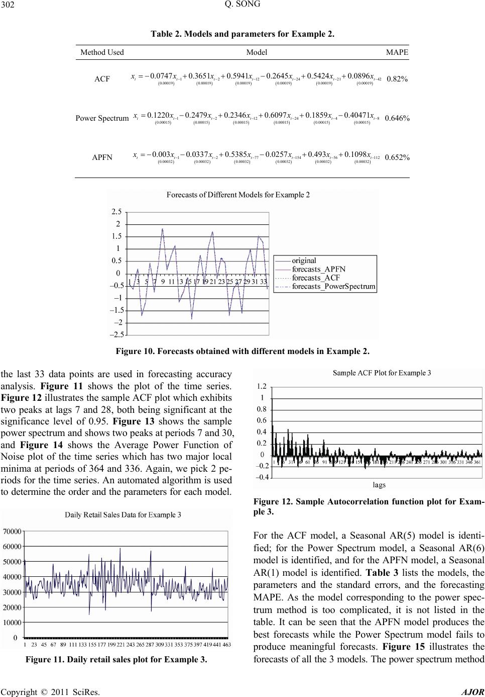

Q. SONG
302
le 2. Models and parameters for Example 2.
Method UsedM
Tab
odel MAPE
ACF t
  
1 2 12242142
0.00019 0.000190.000190.000190.000190.00019
0.0896
tttttt
0.0747 0.3651 0.59410.26450.5424
x
xxx xx x
 
 0.82%
Power Spectrum8t
 
1212244
0.00015 0.000150.000150.000150.000150.00015
0.12200.24790.23460.60970.18590.40471
tt tttt
x
xxxxx
 
  x

0.646%
APFN
 
1277154 56112
0.00032 0.000320.000320.000320.000320.00032
0.003 0.03370.53850.02570.4930.1098
ttt tttt
x
xxx xx
 
x

0.652%
Figure 10. Forecasts obtained with different models in Example 2.
the last 33 data points are used in forecasting accuracy
analysis. Figure 11 shows
Figure 12 illustrates the sample ACF plot which exhibits
the plot of the time series.
two peaks at lags 7 and 28, both being significant at the
significance level of 0.95. Figure 13 shows the sample
power spectrum and shows two peaks at periods 7 and 30,
and Figure 14 shows the Average Power Function of
Noise plot of the time series which has two major local
minima at periods of 364 and 336. Again, we pick 2 pe-
riods for the time series. An automated algorithm is used
to determine the order and the parameters for each model.
Figure 12. Sample Autocorrelation function plot for Exam-
ple 3.
For the ACF model, a Seasonal AR(5) model is identi-
fied; for the Power Spectrum model, a Seasonal AR(6
model is identified, and for the APFN m
AR(1 , the
parameters and the standard errors, and the forecasting
MAPE. As the model corresponding to the power spec-
trum method is too complicated, it is not listed in the
table. It can be seen that the APFN model produces the
best forecasts while the Power Spectrum model fails to
produce meaningful forecasts. Figure 15 illustrates the
forecasts of all the 3 models. The power spectrum method
)
odel, a Seasonal
) model is identified. Table 3 lists the models
Figure 11. Daily retail sales plot for Example 3.

303 Q. SONG
Figure 13. Plot of power spectrum for Example 3.
evidently detects an incorrect period, 30, and this incor-
rect period causes the modeling algorithm to produce a
6th order model to fit the data, and fails to produce good
forecasts in the end with a MAPE of 33.08%. This illus-
trative example indicates the significance of using the
right periods in modeling and forecasting seasonal time
series.
6. Conclusions and Discussions
In this paper, the definition of Average Power Function
of Noise (APFN) has been proposed, and properties of
such a function have been discussed. The most important
property of APFN is that it has a local minimum at the
time lags which are the periods of a seasonal time series.
The numerical examples have exhibited the merits and
the power of APFN in detecting periods in seasonal time
series. ACF and power spectrum are proven to be pow-
erful instruments in signal analysis and many other are-
nas. They may not be the best instruments in detecting
periods for seasonal time series because, as pointed out
Figure 14. Plot of average power function of noise for Ex-
ample 3.
Figure 15. Forecasts obtained w
Table 3. Models and pa
Method Used
ith different models for Example 3.
rameters for Example 3.
Model MAPE
ACF
0.332 0.0940.035xxxx
 

 
 
123 45714
0.0062 0.00620.00620.00620.00620.00620.0062
2128 35 56
0.008890.0062 0.0062
0.03020.108 0.2340.065
0.01670.25890.0290.0720.139
tttt tttt
t ttt
xxxx
xxxxx
   
 


 
84 112 140
0.0062 0.00620.0062
0.065 0.059
tt
xx

 7.89%
t
 0.0062
Power Spectrum Too complicated to list 33.08%
APFN t5.36%
 
1 364 336
0.0111 0.01030.0101
0.247 0.43040.2623
tt t
xx xx

 

Q. SONG
304
at the beginning of the paper, the detected periods of a
seasonal time series should be the ones at which the time
series repeats with the smallest discrepancy, not neces-
sarily the ones at which it repeats the most frequently.
The results of seasonal time series forecasting depend on
not only the model but the periods of the time series as
well. Forecasts are very sensitive to the periods detected
and used in the model. If periods are not properly chosen,
one may end up with high order models and inferior
forecast results. From the empirical examples, it is quite
evident that properly detected periods of a seasonal time
series almost always accompany low order model and
superior forecasts, and APFN consistently produces the
lowest order models in the three illustrative examples.
Therefore, the significance of properly detected periods
cannot be overemphasized
seasonal time series.
As discussed at the beginning of t
pow methods could lead to conflicting results
in detecting periods for the same data set. For that reason,
it will be difficult to automate the detection algorithm
with And power spectrum plots. However, it is rela-
tively simple and easy to automate the period detection
algorithm using APFN. Such an algorithm will involve
selecting the first few lowest local minima, by sorting the
lon ascent order.
The APFN is in the form of square of discrepancy.
Differrms of discrepancy are also possible and
ould opted. For example, the following two dif-
rent forms can be considered in lieu of APFN:
7. References
[1] P. Cortez, M. Rio, M. Rocha and P. Sousa, “Internet Traf-
fic Forecasting Using Neural Networks,” 2006 Interna-
tional Joint Conference on Neural Networks, Vancouver,
16-21 July 2006, pp. 2635-2642.
[2] A. M. De Livera and R. J. Hyndman, “Forecasting Time
Series with Complex Seasonal Patterns Using Exponen-
tial Smoothing,” Working Paper, Department of Econo-
metrics and Business Statistics, Monash University, 2009.
[3] P. G. Gould, A. B. Koehler, J. K. Ord, R. D. Sny der, R. J.
Hyndman and F. Vahid-Araghi, “Forecasting Time Series
with Multiple Seasonal Patterns,” European Journal of
Operational Research, Vol. 191, No. 1, 2008, pp. 207-
222. doi:10.1016/j.ejor.2007.08.024
[4] B. J. Morzuch and P. G.en, “Forecasting Hospital
rivals,” 26th Annual Sympo-
sium on Forecasting, Santander, June 11-14 2006.
rison of Univariate Time Series
Methods for Forecasting Intraday Arrivals at a Call C
” Management Science, Vol. 54, No. 2, 2008,
265. doi:10.1287/mnsc.1070.0786
in modeling and forecasting
his paper, ACF and
er spectrum
CF a
cal minima in a
ent fo
be adc
fe
  
MAD limd
2
T
TT
xt xt
Et
T











  
 
MAPE limd
2
T
TT
xt xtxt
Et
T





 





However, it might be quite difficult to conduct theo-
retic analysis based on those two for ms.
It must be admitted that the results presented in this
paper are quite rudimentary. Further efforts should be
made in order to have a better understanding of the prop-
erties of APFN. One of the issues around APFN is its
connection to ACF and power spectrum. In other words, in
the frequency domain, what do we know about APFN?
All
Emergency Department Ar
[5] J. W. Taylor, “A Compaen-
pp. 253-ter,
[6] J. W. Taylor, L. M. de Menezes and P. E. McSharrA
Comparison of Univariate Methodsor Forecastin-
tricity Demand up to a Day Ahead,” International Jour-
nal of Forecasting, Vol. 22, No. 1, 2006, pp. 1-16.
doi:10.1016/j.ijforecast.2005.06.006
y, “
g Elec f
aylor, “Short-Term Electricity Demand F
ing Using Double Seasonal Exponential Smoothing,”
Journal of Operational Research Society, Vol. 54,
2003, pp. 799-805. doi:10.1057/palgrave.jors.2601
[7] J. W. Torecast-
, No. 8
589
[8] J. W. Taylor, “Triple Seasonal Methods for Short-Term
Electricity Demand Forecasting,” European Journal of
Operational Research, Vol. 204, No. 1, 2010, pp. 139-
152. doi:10.1016/j.ejor.2009.10.003
[9]
in Time
2001.
[11] P. Stoica and R. Moses, “Spectral Analysis of Sials,”
Pearson Prentice Hall, New Jersey, 2005.
[12] Q. Song and A. O. Esogbue, “A New Algorithm for
Automated Modeling of Seasonal Time Series Using
Box-Jenkins Techniques,” International Journal of In-
dustrial Engineering and Management Systems, Vol. 7,
G. E. P. Box, G. M. Jenkins and G. C. Reinsel, “Time
Series Analysis,” 3rd Edition, Prentice Hall, New Jersey,
1994.
[10] D. Pena, G. C. Tiao and R. S. Tsay, “A Course
Series Analysis,” John Wiley & Sons, Hoboken,
gn
No.1, 2008, pp. 9-22.