Optimal Generator Portfolio in Day-Ahead Market under Uncertain Carbon Tax Policy

doi:10.4236/ajor.2011.14031

Paper Menu >>

Journal Menu >>

American Journal of Oper ations Research, 2011, 1, 268-276

doi:10.4236/ajor.2011.14031 Published Online December 2011 (http://www.SciRP.org/journal/ajor)

Optimal Generator Portfolio in Day-Ahead Market under

Uncertain Carbon Tax Policy

Shengyuan Chen1, Ming Zhao2

1Department of Mathem at i c s an d St at i st i cs , York University, Toronto, Canada

2SAS Institute Inc., Cary, USA

E-mail: chensy@mathstat.yorku.ca, Ming.Zhao@sas.com

Received August 26, 2011; revised September 24, 2011; accepted Oct ober 12, 2011

Abstract

The global liberalization of energy market and the evolving carbon policy have profound implication on a

producer’s optimal generator portfolio problem. On one hand, the daily operational flexibility from a well-

composed generator portfolio enables the producer to implement a more aggressive bidding strategy in the

liberalized day-ahead market on a daily basis; on the other hand, the evolving carbon policy demands the

long term robustness of a generator portfolio: it should be able to generate stable cash flow under different

stages of the evolving carbon tax policy. It is computationally very challenging to incorporate the daily bid-

ding strategy into such a long term generator portfolio study. We overcome the difficulty by a powerful ver-

tical decomposition. The long term uncertainty of carbon tax policy is simulated by scenarios; while the daily

electricity price fluctuation with jumps is modeled by a more complicated Markov Regime Switching model.

The proposed model provides the senior executives an efficient quantitative tool to select an optimal genera-

tor portfolio in the deregulated market under evolving carbon tax policy.

Keywords: Carbon Tax, Generator Portfolio, Markov Regime Switching Model, Stochastic Programming,

Unit Commitment, Simulation

1. Introduction

This paper analyzes the impact of the evolving carbon

tax and market deregulation on a thermal power’s opti-

mal generator portfolio. In a centralized market, a gen-

erator portfolio is optimized towards minimizing produc-

tion cost under the constraint that the dynamic demand

must be satisfied. The optimal generator portfolio prob-

lem has been extensively studied under the centralized

market environment. Under this environment, an optimal

portfolio typically include a significant portion of base

load generators and certain amount of peak load capacity.

However, in a decentralized market, satisfying demand is

not a hard constraint anymore. Instead, a power producer

competes in the day-ahead market to maximize their

profit. Bidding strategy, rather than satisfying demand,

turns out to be a critical component in a power producer's

business. Carbon tax also brings a new dimension into

the study since a traditional base load generator is not as

cost effective as before if the carbon tax imposes a high

environment fee. Carbon tax has been piloted in some

jurisdictions, however, the timing, stringency and in-

struments are evolving. New technologies to reduce car-

bon foot print of thermal generators have also been in-

vented and must be included in a current study of the

optimal generator problem, as well as the scenarios of

carbon tax and the bidding strategies.

In a day-ahead market, producers and consumers sub-

mit hourly multiple price and quantity pairs, which are

used to construct a bidding curves by linear interpolation.

We assume that every producer bids all capacity in one

of more pairs at increasing prices of its choices. The ISO

(Independent System Operator) computes the clearing

price for each hour based on the submitted production

and consumer bids. The market-clearing price is used to

pay any accepted production bid and is also the price

paid by any accepted demand bid. In such a situation, the

profit maximization problem faced by a producer de-

composes into independent subproblems for each gen-

erator owned by the producer, see [1]. However, the op-

timal generator portfolio has to be considered in integrity

due to two reasons: capital investment is shared by dif-

ferent generators; and characteristics of generators are

complementary under different policy and price scenar-

269

S. Y. CHEN ET AL.

ios.

We analyze the classical problem under the new envi-

ronments from the perspective of a single price-taker

producer, and we make an important assumption that the

producer has no power to alter the market clearing price.

This pool-based electricity market has also been assumed

in [2,3] as well. In contrast, in a study of market equilib-

rium, one must assume that the collective effort of all

producers will change the market price. [4] makes this

assumption and derives an optimal portfolio for the mar-

ket, instead of an individual producer. Other studies of

the optimal generator problem have different focuses, for

example, [5] considers a multiple objective model; and

[6] put emphasize on a risk adjusted mean return model.

The paper is organized as the followings: Section 2

presents our stochastic optimization model; Section 3

models the bidding strategy of a price-taker producer;

Section 4 is devoted to modelling the stochastic process

underlying the problem of study, and is divided into

three subsections addressing electricity price, natural gas

price and carbon tax separately; Section 5 establishes the

decomposition theorem, which is the foundation of the

proposed methodology. Finally, we conduct a case study

in Section 6 to demonstrate the efficiency of our algo-

rithm using real market data from Ontario, Canada.

2. Stochastic Optimization Model

We consider the optimal generator portfolio for a long

but fixed period consisting of D days. Within this

planning horizon, we are uncertain about the carbon tax

, electricity price



and natural gas price



. We use

a set of scenarios to represent the uncertainty.

S: set of carbon policy scenarios;



: set of natural gas price scenarios;



: set of electricity price scenarios;



: combined random vector





,,r







S: set of scenarios for



: r

SSS





The set of generator technologies and the planning ho-

rizon is described by the following notations:

;

: set of generator types;

D: capital cost of generator ; iI

: set of days in the planning horizon;

: set of months in the planning horizon;

: set of days in the mth month;

Let i

be the percentage of investment for the gen-

erator type , then the vector

represents the genera-

tor portfolio. The portfolio

is subject to the following

budget constraint:





. (1)

We request that the generator portfolio must be able to

generate a minimum monthly cash flow m

. Let





x: cash flow on day from a generator portfo-

lio

under a scenario

;





di i

x: cash flow on day from the generator

in a portfolio

d i

under the scenario

then

()







S mM, , (2)

imposes this single-sided cash flow risk control. A mini-

mum cash flow is often required by many financial in-

stitutions a indicator that its customers are at good finan-

cial status.

Our goal is to maximize the expected profit of a gen-

erator portfolio in the planning horizon. Since this is a

long-term planning problem, we discount the future

profit to its present value. Using discounting factor



the net present value (NPV) of the cash flow from a

portfolio

under a scenario

can be calculated as





NPV xfx











, (3)

Assuming zero salvage value of all generators at end

of planning horizon for simplicity, we can model the

optimal generator portfolio problem as:



maxNPV ,



, (4)

where the expectation



NPV ,









NPV

is numerically

approximated by sS





with scenarios

of weight

The calculation of d

is complicated by the bidding

strategy of the power producer. In the centralized market,

one might calculate the revenue as price times the de-

mand. However, in a day-ahead market, a producer sub-

mits bids to an independent system operator (ISO) in the

previous day, and can only sell the amount indicated on

the bidding result returned from the ISO. As a result, it is

not only the generator’s maximum output rate determines

the revenue; the producer’s bidding strategy also jointly

determines its cashflow. Intuitively, an intelligent bid-

ding strategy can facilitate cashing in a generator’s pro-

duction capability, thermal efficiency and the portfolio's

structural flexibility. To quantitatively establish the rela-

tion between the bidding strategy and the generator

portfolio, i.e., the function



x, we explicitly model

the optimal bidding strategy of a price-taker producer in

the next section.

3. Model the Bidding Behaviour

In [7], a producer’s bidding strategy is divided into three

steps: forecast the next day electricity price; solve a self-

scheduling problem; derive a bidding combination from

S. Y. CHEN ET AL.

270

the optimal solution of the self-scheduling problem. [7]

shows that the bidding strategy achieves a satisfactory

performance in a price-taker pool market. We assume the

producer will follow the strategy consistently. In this

strategy, the producer is also assumed to have a price

forecasting model.







: bidding strategy as a function of known in-

formation;

est



: producer’s estimate of the next day electricity

price;

est



: producer’s estimate of the next day natural gas

price;

com



: market clearing price of the next day electricity;



est



com

hi : producer’s bidding production plan for gen-

erator for hour ;



hi : producer’s committed production as re-

quired by the bidding result from ISO;

tru



: next day true natural gas price;

As pointed out in [7], for a price-taker producer, the

bidding problem can be decomposed into profit maximi-

zation problems for each generator owned by the pro-

ducer. After forecasting the next day electricity price

est



, the producer solves a self-scheduling problem for

each generator :



,,, 1

max ,

subject to ,,,

Hest esti

hi h

esti ii

pzvy

ttt

est iiii

hih hh

pcx

pzvy x









 (5)

where



i is the feasible operating region for the

generator . We model the feasible operation region

using a set of mixed linear integer constraints as in [7],

which outlines the power output limit, ramping rate, and

minimum up and down time, see [7] for the formulations.

[8] shows that hedging performance and consequently

the income from production strongly depends on the

flexibility of its generation facility, i.e., the feasible re-

gion described in





. In this self-scheduling prob-

lem, is the production cost for the hour and is

composed of the shutdown cost , start-up cost ,

fixed cost

, fuel cost and the emission cost

h, where and are baseline fuel cost rate

and emission rate of the technology :

ii es

hbp



re est



iiiiiii esti ie

hhhhhh

cCzAvSy brep



 



. (6)

z, and

are the indicator variables correspond-

ing to each of the listed events. In (6), the production

cost is linear with the production amount. We also ob-

serve that a larger generator costs more to startup and

shutdown, and incurs higher fixed cost.

After solving the self-scheduling problem, the pro-

ducer shall make a bidding combination to maximize its

chance of getting the optimal self-scheduling production

plan from ISO, see [7] for details on the bidding strategy.

The strategy enables the producer to generate the optimal

amount from its self-scheduling model with a pre-speci-

fied confidence level, provided that the mean and vari-

ance of the producer’s price forecasting model are cor-

rect. On the day of delivery, the producer will re-optimize

its production plan based on the bidding result and the

current price information:



,, =1

max ,

subject to ,,

Hcom comi

hi h

iii

zvyh

hhh

ii ii

hh h

zvy x







 (7)

where





,,,,

com comcom com

iiHi Hi









(8)

are the bidding result and the cost function



iiiiiii truiico

hhhhh hh

cCzAvSy birep



 ,

uses the updated price information. Note that the pro-

ducer only submits feasible bids in (5), hence the prob-

lem (6) is always feasible. Hence the true cash flow of

the generator i in a portfolio

on day under

scenario

is:



com comi

di ihih







 (9)

Note that the relationship between the cash flow





di i

x and a portfolio

is determined by the com-

plicated forecasting and bidding procedures of a power

producer. Though it is impossible to write





di i

x as an

elementary function of

, it is straightforward to simu-

late it: for a given a portfolio

and a scenario





sss



, one can mimic the producer's decision

process as the following:

1) forecast the electricity and natural gas price to get





est est



;

2) solve the self-scheduling problem (5) to get ;

est

3) follow the bidding strategy in [7] and return the

bidding result using

com



as tru



;

4) adjust the production plan by solving (7) using



as tru



in computing ;

5) calculate





di i

x for all , and let iI









ddii



fx



4. Model the Uncertainties

4.1. Electricity Price Uncertainty

In a day-ahead market, clearing price for each hour could

be modeled as a random variable. Especially, the charac-

teristics of seasonality on annual and weekly level, mean-

271

S. Y. CHEN ET AL.

reversion and jumps should be appropriately reflected.

The infrequent but large jumps caused by extreme load

fluctuation such as severe weather, generation outage or

transmission failure, make the energy market quite dif-

ferent from a financial market. Though this paper is not a

research on modelling electricity price, its importance for

this research is evident: only under a properly generated

set of pricing scenarios, one can correctly evaluate the

performance of a generator portfolio.

There are extensive research on how to generate elec-

tricity price scenarios. For example, Markov regime

switching model has been proposed in [9,10] develops a

pure mean-reversion model with the capability to create

jumps; the jump diffusion/mean-reversion model is stud-

ied in [11]; neural network is used to predict prices in

California in [12]. A comprehensive review article in this

field appeared in [13]. Here we use Markov regime

switching model due to its flexibility in modelling the

jumps.

A jump in electricity price can be considered as a

change from the base regime to the spike regime in a

two-regime model. The switching itself is modeled as a

Markov chain. Let indicate the base regime, and

indicate the spike regime, the Markov transition

matrix contains the probabilities of switching

between the two regimes:

R

RPij

11 11

22 22

Ppp











In a Markov process, the probability of regime at

time starting from state at time equals

tmi t



Now we demonstrate how to use Markov switching

model in a particular market. Given a set of historical

price data 17

for W weeks, the first step is to

de-seasonalize the data by fitting a deterministic nonlin-

ear seasonality model [13]:

,,W

pp



2π

sin 24

2π

cos,

8760

Sh h









 















(10)

where

1if hour is in weekend or holiday

0otherwise.

D



 (11)

Here the 1



, 2



capture the intra-day change,



describes the change of weekends and holidays, and 1



reflect the annual periodicity.



In a second step, after we get the optimal estimates of

parameters



, 1



, 2





, 1



, , we compute the

de-seasonalized log-price:





log





We model the de-seasonalized log-price using the

Markov regime switching model [9]. Under this model,

one can flexibly choose a stochastic process to describe

the log-price in the spike regime, yet another stochastic

process to describe the log-price in the base regime.

Usually a different stochastic process is chosen to model

the jumps in the spike regime. We model the log-price in

the base regime as a mean-reversion process, i.e.,





YYh

 

 d

The drift term







 is negative if the electric-

ity price is higher than the mean 1



and positive if it is

lower. Hence the drift term drags the price back to its

mean value 1



in the long run, with



describing the

speed of reverting to the mean value. The stochastic term

is the increment of the standard Brownian motion,

and is multiplied by the market volatility



We model the log-price in the spike regime as a log-

normally distributed random variable, i.e.,





log h

follows a normal distribution









. The mean 2



usually higher than the mean 1



ofhe base regime.

The 2



corols the magnitude of the spikes. nt

Finally, we estimate the parameters (







,11,22 ) using the de-seasonalized historical

log-price data. The estimation is quite involved, but is

clearly documented in [14]. Using true historical data

from a specific market, one may capture the market

characteristics: frequency and magnitude of jumps,

means and variances of the price in the two regimes, and

the speed of mean-reversion in the base regime.

p p

4.2. Natural Gas Price Uncertainty

As many countries and regions have planned to abandon

the coal generators in near future, natural gas prices be-

come one of the most important factors in deciding the

optimal generator portfolio. We model the natural gas

price as a Brownian motion with positive drift:

ddd









 (12)

And we model the coal price as constant since its

volatility is relatively low.

4.3. Carbon Tax Uncertainty

To correctly evaluate the performance of a generator

portfolio, we need a comprehensive set of carbon tax

scenarios as well. Carbon tax uncertainty does naturally

follow a stochastic process as the natural gas price or the

electricity price. Instead it is a complicated movement

S. Y. CHEN ET AL.

272

programming model since



x can only be evaluated

by steps (1)-(5) in the Section 3. A natural choice is to

conduct a simulation optimization research, where we

equip a power producer with a generator portfolio 0

and let it act as a smart agent following steps (1)-(5) in

the Section 3. At end of such a simulation, one get a cor-

responding NPV for the generator portfolio 0

. To get

an expected NPV for the portfolio 0

, one repeats the

process for each scenario in a large sample





,1,,



. A simple simulation optimization algo-

rithm calculates the



ENP

for many different gen-

erator portfolios i

, 1, ,iN



 (tries), and at end

picks the portfolio with the highest ENPV. A sophisti-

cated simulation optimization algorithm may conduct

more intelligent search for better i

, see [15] for such

an advanced searching algorithm. needs to be large

for a simple simulation optimization procedure to ensure

sufficient coverage. does not need to be huge for a

sophisticated procedure, however it is non-deterministic

in general. For both cases, optimality of

can not be

guaranteed. The computational burden is prohibitive as

we need to solve the producer’s self-scheduling problem

(5) for times for each scenario



and portfolio

, which brings the total to . Considering a

30 year problem with

DSN

10950D



, a moderate number of

scenarios 26S



, and 1000N



tries, the total num-

ber of self-scheduling problem to be solved is 284,700,000.

We note that each (5) is a hard mixed integer linear pro-

gramming (MIP) problem, and we haven’t counted the

adjusting problem (7) and other steps listed in the section

3 yet. This computational burden makes the optimal

generator portfolio problem with daily bidding details

practically intractable.

driven by economical and political forces. In a practical

implementation, one could follow advices from policy

analysts and generate most likely scenarios for the local

jurisdiction. In this study, we create the following dis-

crete model for simplicity: 1) there are equal probability

of implementing a carbon tax in T, , , ,

years away from now; 2) if a carbon policy has not

been adopted years from now, then the conditional

probability of adopting it later is updated to

2T3T4T

5TiT





15 i



Following this conditional probability updating scheme,

if a carbon policy has not been implemented years

from now, then the chance of implementing it at is

one, which respects our believe that a carbon policy will

be implemented sooner or later. 3) the carbon tax rate

could be high with a probability high or low with a

probability high for each possible implementation.

Once a carbon policy with rate

p r



is implemented, we

assume it remains constant in the planning horizon of

this study. Figure 1 shows all carbon tax possibilities of

this discrete model.

We note that some states/provinces in North America

have implemented pilot carbon tax and in Europe the

carbon emission is traded in the CO2 market; however,

carbon policy is evolving and the associated uncertainty

remains a big factor in optimal generator portfolio prob-

lem.

To generate a scenario





sss







,,r

, one follows

the models in 4.3, 4.2 and 4.1 separately. This implicitly

assumes independence among





. We acknowl-

edge that the possible increase of electricity price due to

a change in fuel price can only be captured by a very

complicated macro-economic model, which is out of the

scope of this paper. However, it seems evident that the

technological substitution has more elasticity than the

electricity demand, which justifies our approach as we

focus on the dynamics of the optimal composition of

technologies under the changing carbon tax and fuel

prices.

To overcome this difficulty, we prove a useful theo-

rem, which allows us to evaluate for



f1dD



\iniI



only once; and find an optimal generator

portfolio *

by solving a simple linear programming

model.

Theorem 5.1 (Decomposition theorem) The cash

flow of a generator portfolio depends on the capacity of

individual generators linearly , i.e.,

5. Computational Tractability

The optimal generator portfolio decision model (4) with

constraints (1) and (2) is not an usually mathematical





ddi





x



Figure 1. The diagram shows two possible outcomes of carbon tax rate (high or low) at each of the five calendar years shown

in the graph, which brings the total number of carbon tax scenarios to ten in this study. A filled circle represents the event

hat a low tax rate is implemented in the associated year. t

S. Y. CHEN ET AL. 273

Proof. As shown in [7], in the price-taker bidding

strategy, the performance of each generator in a portfolio

can be evaluated independently, i.e.,





x.

It remains to show that







si x

didi i

xfx. The con-

clusion follows the linearity of the objective function and

the feasible region in producer’s bidding step (5), ad-

justing step (9) and the cash flow formula (9).

Following Theorem 5.1, one only needs to evaluate

for a “standard” generator with capacity 1, and



compute





idi

dD sS







 and



mi di



s

f. Then the optimal generator portfo-

lio model (4), subject to constraints (1) and (2) is equiva-

lent to the following linear programming problem:



max

s.t. 1

iii

xiI

mii im

gxk

xkfs Sm M





 



(P)

In the above model, ii

k gives the capacity of gen-

erator type for

amount of investment.

6. Case Study

We use the historical hourly electricity price data of the

Independent Electricity System Operator of Ontario from

February 18th 2009 to April 2nd 2010 to fit the Markov

regime switching model, and the fitted parameters are

shown in the Tables 1 and 2. We generate the natural gas

price scenarios following the equation (12). The carbon

policy scenarios are generated from the discrete model in

subsection 4.3 with the five discrete years being 2015,

2020, 2025, 2030, and 2040. We let 23

high

p,

$200

high

rtCtC



and . A total of 26 identi-

cal and independently distributed (i.i.d.) samples of

$50

high

r



sss



 are generated. Two electricity price

sample paths are shown in Fi gure 2.

We use three types of thermal generators , ,

in this study. The technological parameters, compiled

CGT

Table 1. De-seasonality parameters.









0.00012 17.36 –33.13 7.87 –2.38 –33543

Table 2. Markov switching model parameters.







0.0471 3.48 1.51 0.03 0.139 0.09 0.41

(a)

(b)

Figure 2. Two scenarios of hourly Ontario Electricity Price

for 30 years. x-axis represents number of days, and y-axis

indicates the electricity price. (a) Scenario a; (b) Scenario b.

from [16,17], are representative for a typical coal gen-

erator, a natural gas generator and a combined gas tur-

bine. In Table 3 , we list the following technical parame-

ters: minimum power output P, maximum power out-

put P, start-up ramp limit , shutdown ramp limit

, ramp-up rate limit , ramp-down rate limit ,

minimum up time and minimum down time .

In Table 4, we give the following cost parameters: capi-

tal investment per unit of capacity , fixed operating

cost

SD RU RD

DTUT

, start-up cost , shutdown cost , baseline

fuel cost (at current natural gas price $ 8/GJ), emis-

sion rate . Note that the baseline fuel cost implicitly

Table 3. Generator technological parameters.

PPSUSD

D UT DT

MWMWMW/h MW/h MW/h MW/h h h

C20043080 70 30 20 2323

G112294170 160 80 70 4 4

T180450155 134 76 59 8 7

S. Y. CHEN ET AL.

274

Table 4. Generator economic parameters.

Capital Fixed Starup Shutdown Fuel Emission

$/kW $/kW $ $ $/kW kg-C/MWhr

C 1200 22 1038 56 5 228

G 450 15 230 21 10 89

T 1550 26 549 40 9 27

reflects the thermal efficiency of a generator. To get the

fuel cost rate for generator at h, one just need to

multiply



with the corresponding baseline fuel

cost.

We let the natural gas price 1$8GJ



,

$1.2 10GJ





 , 4

$2.1 10GJ







 , which ap-

proximate the current market price and the hourly drift-

ing rate.

We set the minimum cash flow 30

f for each

month. In practice, this minimum profit level should be

set according to the producer’s business and financial

status. Also note that the constraint (2) could be read as

if the portfolio worths $ 1 investment, hence the monthly

minimum cash flow level should be set for this $ 1 port-

folio.

The computation is conducted on a personal computer

with 2.13 GHZ Intel Core 2 Duo and 2 GB 800 MHZ

DDR2 SDRAM. We used MATLAB to generate scenar-

ios, fit parameters and evaluate

, and used GLPK/

GMPL for modelling the self-scheduling problem (7),

adjusting problem (5) and the portfolio selection problem

(P). Most tasks took negligible time, except evaluating

for the 26 scenarios, 3 generators and 10950 days,

which requires solving 1,708,200 MIP problems, see (7)

and (5). These problems are not related and can be

solved in parallel. A simple serial code written in ANSI

C solved all these MIP problems in 9 hours. The portfo-

lio selection problem (P) has three decision variables,

one budget constraint (1), and 9360 minimal monthly

cash flow constraints (2), is solved to optimality in three

seconds. In the contrast, a simple simulation optimization

method with 1000 tries, would need 9000 hours to de-

liver a suboptimal result.



The optimal solution *

from our linear program-

ming model (P) is:

 0%C, 8%G, 92%T in terms of capital

value; or

 0%C, 23%G, 77%T



in terms of capac-

ity,

where stands for carbon, for natural gas and

for combined gas turbine.

C GT

The result clearly shows that though coal generator

technology has lowest production cost, the prohibitive

environmental fee in some high carbon tax scenarios

makes it unfavourable. If one assumes that high carbon

tax has a high possibility as this model does, then the

coal generators should not show up in an optimal portfo-

lio. The combined gas turbine and natural gas generator

exhibit complimentary features under different scenarios,

and the optimal solution recommends the 23/77 combi-

nation. The result might change if a drastically different

carbon tax model is applied. A decision maker may sup-

ply the model with a different perspective of the carbon

tax policy and gain a different optimal portfolio.

The daily simulation for a “standard” generator over

30 years also reveals some insightful phenomena. We

show two of such simulations in 1. The subgraph (a)

shows a scenario where the high carbon tax is imple-

mented in 2015; and the subgraph (b) shows a scenario

where a low carbon tax is implemented in 2025. We first

observe that the order of performance of the three gen-

erator technologies could change significantly after the

carbon tax. The coal technology (blue line) clearly out-

performs the other two technologies before the carbon

tax, but after the carbon tax, it yields negative cash flow

in scenario (a) and ranked in a second place in the sce-

narion (b). Secondly, many downward cashflow jumps

dominates both subgraphs (a) and (b). A careful drill

down analysis shows that these are caused by inaccurate

electricity price forecast. Historical electricity price also

shows many jumps due to many unpredictable events

including network congestion. The Markov regime

switching model can generate these jumps, thus mimick-

ing the price pattern. However, forecasting these jumps

at daily level can only be accurate in a statistical sense at

the best, hence a power producer’s daily forecast error is

unavoidable. As a result the submitted bids could be far

off the true optimal production plan, hence the flexibility

of adjusting the production plan is necessary. This phe-

nomena further emphasize the importance of studying

the long term planning problem with the daily bidding

details. Without this “nano” level investigation, a sig-

nificant profit loss due to the unavoidable price jump

cannot be correctly captured and evaluated. Finally, we

note that natural gas generator has less downward cash

flow jumps, and the occurred jumps are small in magni-

tude. We contribute this to the technology’s flexibility.

In our drill down analysis, the natural gas generator tech-

nology allows more flexible production adjustment when

the forecast is not accurate. As shown in the Figure 3,

this flexibility shapes the cash flow pattern

of dif-

ferent technology drastically, and yields tremendous

loss savings in the planning horizon under study.

7. Conclusions

Though it is widely accepted that the market deregula-

tion and the evolving carbon tax have profound impact

on an optimal generator portfolio, it is challenging for

275

S. Y. CHEN ET AL.

(a)

(b)

Figure 3. x-axis shows days and the y-axis shows cash

flow . Blue line for the coal generator, magenta line

for natural gas, and cyan line for the combined gas turbin.

(a) High carbon tax since 2015; (b) Low carbon tax since

2025.



senior executives to make a quantitative decision analy-

sis, i.e., what’s the optimal percentage for each generator

technology? The proposed model incorporates into con-

sideration the important day-ahead bidding activity, and

three major uncertainty sources underlying the decision

problem. For such a long term planning study, these me-

ticulous considerations at daily operation level usually

lead to computational intractability. We overcome this

difficulty by vertically decomposing the problem into

individual “standard” generator of capacity one, and

convert the problem into a simple linear programming

model. We are able to compute the proposed model on a

personal computer within a reasonable time limit. The

result shows that the daily negative cash flow jumps are

dominating, and constitute a significant part in evaluat-

ing the ENPV of a portfolio. Once supplied with the

market and candidate generator parameters, together with

the carbon tax scenarios of the local jurisdiction, a deci-

sion maker can apply the model and the decomposition

algorithm to find an optimal generator portfolio effi-

ciently.

8. References

[1] J. M. Arroyo and A. J. Conejo, “Optimal Response of a

Thermal Unit to an Electricity Spot Market,” IEEE

Transactions on Power Systems, Vol. 15, No. 3, 2000, pp.

1098-1104. doi:10.1109/59.871739

[2] ISO New England Inc., Technical Report, 2002.

http://www.iso-ne.com

[3] ERCOT, The Electric Reliability Council of Texas, Inc.,

Technical Report, 2002. http://www.ercot.com

[4] J. Hinz, “Optimizing a Portfolio of Power-Producing

Plants,” Bernoulli, Vol. 9, No. 4, 2003, pp. 659-669.

doi:10.3150/bj/1066223273

[5] N. M. Pindoriya, S. N. Singh and S. K. Singh, “Optimal

Generation Portfolio Allocation in Competitive Electric-

ity Market,” Annual IEEE India Conference, Gujarat,

18-20 December 2009, pp. 1-4.

doi:10.1109/INDCON.2009.5409351

[6] X. Yin, Z. Y. Dong and T. K. Shaha, “Optimal Portfolio

Selection for Generators in the Electricity Market,” Pro-

ceeding of IEEE PES General Meeting, Pittsburgh, 20-24

July 2008, pp. 1-7.

[7] A. J. Conejo, F. J. Nogales and J. M. Arroyo, “Price-

Taker Bidding Strategy under Price Uncertainty,” IEEE

Transactions on Power Systems, Vol. 17, No. 4, 2002, pp.

1081-1087. doi:10.1109/TPWRS.2002.804948

[8] J. Doege, P. Schiltknecht and H.-J. Lu¨thi, “Risk Man-

agement of Power Portfolios and Valuation of Flexibil-

ity,” OR Spectrum, Vol. 28, No. 2, 2006, pp. 267-287.

doi:10.1007/s00291-005-0005-4

[9] M. Bierbrauer, S. Tru¨ck1, and R. Weron, “Modeling

Electricity Prices with Regime Switching Models,” Lec-

ture Notes in Computer Science, Vol. 3039, 2004, pp.

859-867. doi:10.1007/978-3-540-25944-2_111

[10] M. T. Barlow, “A Diffusion Model for Electricity Prices,”

Mathematical Finance, Vol. 12, No. 4, 2002, pp. 287-298.

doi:10.1111/j.1467-9965.2002.tb00125.x

[11] P. Skantze, M. Ilic and J. Chapman, “Stochastic Model-

ing of Electric Power Prices in a Multi-Market Environ-

ment,” Proceeding of Power Engineering Society Winter

Meeting, Singapore, 23-27 January 2000, pp. 1109-1114.

[12] F. Gao, X. Guan, X.-R. Cao and A. Papalexopoulos,

“Forecasting Power Market Clearing Price and Quantity

Using a Neural Network Method,” Proceeding of Power

Engineering Society Summer Meeting, Seattle, 16-20 July

2000, pp. 2183-2188.

[13] J. J. Lucia and E. S. Schwartz, “Electricity Prices and

Power Derivatives: Evidence from the Nordic Power Ex-

change,” Review of Derivatives Research, Vol. 5, No. 1,

2002, pp. 5-50. doi:10.1023/A:1013846631785

[14] J. D. Hamilton, “Regime Switching Models,” Palgrave

Dictionary of Economics, Palgrave McMillan Ltd., New

York, 2005.

S. Y. CHEN ET AL.

276

[15] L. J. Hong and B. L. Nelson, “Discrete Optimization via

Simulation Using COMPASS,” Operations Research,

Vol. 54, No. 1, 2006, pp. 115-129.

doi:10.1287/opre.1050.0237

[16] C. Wang and S. M. Shahidehpour, “Ramprate Limits in

Unit Commitment and Economic Dispatch Incorporating

Rotor Fatigue Effect,” IEEE Transactions on Power Sys-

tems, Vol. 9, No. 3, 1994, pp. 1539-1545.

doi:10.1109/59.336106

[17] P. S. Reinelt and D. W. Keith, “Carbon Capture Retrofits

and the Cost of Regulatory Uncertainty,” The Energy

Journal, Vol. 28, No. 4, 2007, pp. 101-128.

doi:10.5547/ISSN0195-6574-EJ-Vol28-No4-5
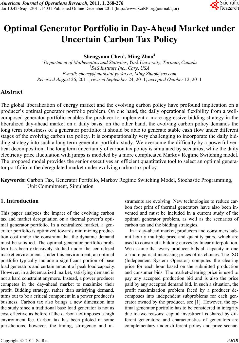