American Journal of Operations Research, 2011, 1, 259-267
doi:10.4236/ajor.2011.14030 Published Online December 2011 (http://www.SciRP.org/journal/ajor)
259
On Fuzzy Random-Valued Optimization
Monga K. Luhandjula
Department of Deci sio n Sci e n ces , Uni versit y of South Africa , Pretori a, South Africa
Received July 27, 201 1; revised August 30, 2011; accepted September 14, 2011
Abstract
In this paper, we propose a novel approach for Fuzzy random-valued Optimization. The main idea behind
our approach consists of taking advantage of interplays between fuzzy random variables and random sets in a
way to get an equivalent stochastic program. This helps avoiding pitfalls due to severe oversimplification of
the reality. We consider a numerical example that shows the efficiency of the proposed method.
Keywords: Fuzzy Random Variables, Random Sets, Fuzzy Stochastic Optimization
1. Introduction
1.1. Background
Fuzzy Stochastic Optimization (FSO) is a worthwhile
topic. It provides a glimpse into joustling with the com-
plex and yet useful issue of handling situations where
fuzziness and randomness are under one roof in a optimi-
zation setting. Here are, without any claim for exhausti-
vity, some examples of concrete problems necessitating
consideration of both fuzziness and randomness: Linear
regression problem in the presence of both random and
fuzzy variables [1]; Renewal processes where inter-arri-
val times are only known as subjective categories of the
form; almost 3 hours, around 2 hours, less than 4
hours…, the occurrence of which cannot be predicted
with precision [2]. An interested reader is referred to [3]
where the terrain covered by FSO is surveyed. The
reader may also consult [4-9] for more insights in this
emerging subfield of mathematical programming under
uncertainty. The presence of both possibilistic and proba-
bilistic information within a mathematical programming
framework is a harbinger of computational nightmares if
one were to approach the problem without any simplifi-
cations. Nevertheless, pitfalls due to severe oversimplifi-
cation of the reality may lead to a bad caricature of the
problem under consideration. In this paper the focus is on
an Optimization model involving fuzzy random coef-
ficients. This model comes up in several applications
including optimal portfolio selection [10], inventory
model [11], water resource management [12]. The com-
monly used approach for solving this model is to craft a
deterministic surrogate of the fuzzy stochastic optimiza-
tion at hand, by exploiting the structure available while
sticking as well as possible to uncertainty principles.
This approximation paradigm is central to the literature
[13-15], although some researchers have questioned both
its robustness and its general validity [16]. Without a
serious output analysis, it is hard to ascertain both the
quality of the approximation and the viability of the
obtained solutions.
1.2. Contribution
In this paper, we establish a mathematical connection
between fuzzy random variables and random sets. This
connection is then used to get an equivalent counterpart
to the original problem. The challenging task of singling
out a solution of the resulting stochastic program with
infinitely many objective functions is also addressed.
The paper contains a systematically solved example
showing the efficiency of the proposed method.
1.3. Notation
Throughout the paper will denote the set of
fuzzy numbers with compact supports. If

cc
F


cc
aF

then a

 is its

-level set that is a closed interval.
With


0,1C
 we will indicate the set of real-valued
bounded f u nct ions f on [0,1] such that:
1) f is left continuous for any


0,1t


0,1 2) f has a right limit for any t

Conventionally, for , and
cc
aF
,
L
aaa








0,1C

 stands for the collections of families





0,1
ZZ



 of closed intervals endpoints of which

M. K. LUHANDJULA
260
are members of


0,1C
. We’ll use the following notatio n
for


Z

;
 
,
L
ZZZ 


.
For the distance between

12 0,1
,C ZZ1
Z
and
2
Z
is given by:


 


1
121 2
0,1 0
,d ,
H
C
dZZ ZZd




where
H
d denotes the Hausdorff metric. Moreover
I
and denote the interval [0, 1] and the indicator
function of A respectively.
1A
1.4. Structure of the Paper
The remainder of the paper is organized as follows. In
the following section, we introduce the notions of random
closed set and fuzzy random variable and we briefly
discuss some of their properties. In Section 3, we prove
that the set of fuzzy random variables can be embedded
into the set of random closed sets isomorphically and
isometrically. This embedding result is then exploited in
Section 4 to describe an approach for solving mathemati-
cal programs with fuzzy random coefficients. Section 5
is devoted to a numerical example for the sake of illus-
tration. We end up in Section 6 with some concluding
remarks along with lines for further developments in this
field.
2. Random Set and Fuzzy Random Variable
2.1. Random Set
Consider a probability space


,,PB and let
F
be a
set of collections of subsets of . A random set in
is a map: E E
F
 that satisfies some measurability
conditions [17]. For our purposes, and we
consider random sets of the form: E


0,1
:
()
C
I
X
X





The class of the above random sets is denoted by


R.


R can be endowed with the following metric
based on the Haus do rff metric
H
d For


,XY R,



  
,d
R
dXYY P

,d
H
IXd





Given we say that

,XY R
X
is less or equal
than , in symbol: Y

R
X
Y


if


,
I


,
 
sup infXY


 .
For details on random sets, we refer the reader to [18,
19].
2.2. Fuzzy Random Variable
Consider again a probability space A map

,,PB


:
cc
XF
X


 

is a fuzzy random variable if for every


0,1   and
for every Borel set B of , where
is defined as follows.


1
XB

B
:2X

 




XxXx


  .
In the sequel, the set of fuzzy random variables in the
above sense is denoted by . A remarkable pro-
perty of a fuzzy random variable (frv) is that Zadeh’s
decomposition principle for fuzzy quantities extends
naturally to frvs, that is for

F


YF

,
 
0,1
YY




.
Another fundamental key fact about fuzzy random
variables, which is of interest on its own right and
which has a huge impact on applications is that an

-level set of a fuzzy random variable is a random
interval [17]. Arithmetic operations on


F

are
defined as follows.
Given


,YZ F

 and

 we have:




YZY Z


 ;






YY

 ⊙;


YZ

if and only if YZ


,


where and ○ indicate that operations are on □


F

and on


cc
F respectively. It is worthmen-
tioning that

and ⊙ are based on Zadeh’s extension
principle [20]. Moreover, YZ


 is tantamount to
IZY




for all (0,1]


where
I
 stands for in-
equality between intervals.
We equip


F

with a distance defined as follows.
Given


,YZ F




 
,d,d
H FI
dYZY ZP
 
d




As in the case of random variables, it is efficient to
describe the distribution of a frv by means of certain
measures summarizing some of its most relevant charac-
teristics. In this way, the first two moments of a fuzzy
random variable are defined as follows. The expecta-
tion of a frv , in symbol is the fuzzy quantity
whose
Y
YEY

-level sets are given by:

261 M. K. LUHANDJULA


d is a selection of EYf P fY



.
The variance of Y, in symbol VY, is given by the
following relation:



,
F
VYEdY EY


Limit theorems [22] have been obtained for frvs based
on the above notions of expectation and variance.
Moreover, fuzzy random variables enjoy the Random-
Nikodým property [21 ]. That is, if


:cc FF  is a
P-continuous fuzzy measure of bounded variation, then
there is such that:

YF

d
B
F
BYP BB,
3. Embedding Theorem for Fuzzy Random
Variables
3.1. Auxiliary Mappings
The following three maps will play a staring role in the
statement and the proof of an Embedding Theorem for
fuzzy random variables.
3.1.1. Mapping 

 maps into as follows.

cc
F

0,1C



 
0,1
:
,
cc C
L
I
F
aa a








 


where

=
L
L
aa



and

=aa




.
It is well known (see e.g [23,24]) that thus defined
is injective, isometric and satisfies the following relation:

For and

,cc ab F

,st

, , 0s0t







11
st
absat






⊙⊙ b


.
3.1.2. Mappin gs f

and


The two other auxiliary maps are given below.
 
:
cc
fF F
XX








0,1
:
C
F
XX


 



3.1.3. Remark
Relationships between auxiliary mappings are shown in
Figure 1. The three auxiliary mappings make the dia-
gram given in Figure 1 commutative.
As a matter of fact,
 


f
XX

 

Figure 1. Diagram involving auxiliary functions.
Therefore of





.
3.2. Main mapping

The mapping

that is used in our Embedding Theorem
for fuzzy random variables is defined as follows.


: FR
XX






where

 
0,1
:
,
C
L
X
XX













and




,,
LL
I
XX XX
 



 


 

Relationships between the main mapping and auxiliary
mappings is given in Figure 2. Mappings involved in Fig-
ure 2 make the diagram given in Figure 2 commut ati ve .
As a matter of fact,
For




  
XXX


 


Hence
X
X


.
For the sake of convenience, we identify a real number
a with the following degenerate fuzzy number.


:0a
,1
with
X

Figure 2. Diagram involving the main mapping.

M. K. LUHANDJULA
262


1if
0otherwise.
ta
at 




Moreover, we denote by , the degenerate
fuzzy random variable:

1AA


1:
1
Acc
A
F
A




Building on the mappings

,
f

,


,

and on
the above terminological conventions, we are now ready
to present the main result of this section .
3.3. Statemen t and Pr oof o f the Embed ding
Theorem
3.3.1. Theorem 1
Consider ;

,XY F

,

, 0

, 0


and let

be as in §3.2. Then the following statements
hold true.
1)

is injective
2)
 

11=
X
YX

Y




 


 
3)




,,
FR
dXYd XY 


4)

R
X
YXY




In other terms

maps


F into isomor-
phically and isometrically.

R
Moreover,

is order preserving.
3.3.2. Proof of Theorem 1
1) Let and assume

,XY F
X
Y

  Then for

 we have that:


 
XY

 ;
 
X
Y

 .
This means that for

 we have:
  

 


f
XX fYY






As is injective, we conclude that

X
Y


 for all
.


Therefore
X
Y and we are done.
2)
























11
11
11
11
11
XY
XY
fXY
XY
XY















 













 
 
 
 













 
 

11
.
XY
X
YX
XYXY



 
 








⊙⊙
Y
Therefore






11
X
YX

Y

 




 
as desired.
3)



 


  

   


d,
d,d
d,d
d,d
R
H
I
H
I
H
I
XY
XYP
XYP
XYP




d
d
d.

 

 














As

is isometric we have that:



 






d,d,d d
d,.
H
I
R
F
XYX YP
XY










4)
X
Y

if and only if
X
Y


,

.
This is tantamount to say that:
X
Y

if and only if
L
X
Y




 ,

  (1)
As L
X
X




 and L YY



, we have that (1)
can be written:
if and only if
,, ,
LL
XY
XX YY
 
 








(2)
(2) is equivalent to
X
Y

if and only if
X
Y

if and only if

  
XY

 ,


(3)
But






XY

 ,

 is equivalent to








sup infXY


   ,

 
or

R
X
Y




.
Therefore (3) can be written:
X
Y if and only if

R
X
Y




and we are done.



4. Solving Fuzzy Random-Valued
Optimization Problems
4.1. Case of Deterministic Feasible Set
Here we are interested in solving the following Optimi-
zation problem:

263 M. K. LUHANDJULA
 
min
1
f
x
PxX






where and

:n fF

X
is a convex and
bounded subset of
n

As

is an isomorphism isometric and order preser-
ving, solving


1P is tantamount to find a solution of
the mathematical program:
 
min
1
f
x
PxX







More form ally we have,
Propositi on 1
*
x
is an optimal solution of


1P if and only if *
x
is an optimal solution of

1P

.
Proof
Assume *
x
is an optimal solution for


1P. Then
*
x
X and


*
f
xfx

x
X

.
Then by Theorem 1 (d) we have that:




*
R
f
xf 



x
x
X
This means *
x
is optimal for .

1P
Assume now that *
x
is optimal for

1P

. Then
*
x
X and


*
f
xf  x

x
X . By Theorem
1(d) again, we have that:


*
f
xfx

x
X
and we are done

By definition of

,

is equivalent to:

1P
L

 


min (,(
1
0,1 ;.
fx fx
PxX







 








Worthy to note here is the fact that is a sto-
chastic multiobjective mathematical program with infini-
tely many objective functions.

1P
To the best of our knowledge, there is no available
solution technique for it. This is the price to pay for
considering an equivalent approach to treat fuzziness
instead of an approximate one. To be able to carry out a
fairly discussion of we find it convenient to assu-
me that:

1P
1) the expectation model is acceptable for tackling
randomness;
2) minimizing an interval can be well handled by mi-
nimizing its midpoint.
It might be pointed out in passing, that assumption 1)
is often used in the literature for derandomization
purposes [25,26]. Moreover, assumption 2) grants us a
way for transforming intervals into real numbers. This
transformation generalizes quite canonically the real case.
As a matter of fact the midpoint of


,aa is . a
Bearing in mind 1), 2) and considering the fact that
multiplying an objective function by a constant does not
alter the localisation of an optimum,

1P

 may be
written as follows.




 



min
2
0,1 ;.
L
Ef xEf x
PxX


















from now on,






fx

stands for



 


Ef xEf x

L

 

Therefore (P2) reads merely:

  
min
2
fx
PxX
I











Let’s now select a finite subset of

1
,=, ,m IS

 
and let 1,,
n

  be real-valued functions such that:
1)


0  
j;
I


;
=1, ,jm
2)

1if
0if
ji
ij
ij






Define a positive interpolating operator K with nodes
1,, m

  as follows:
 

=1
=m
j
j
j
Kh h

 

Consider now the following mathematical programs.



 
min
3
.
Kf x
PxX
I















min
4
1, ,
j
fx
PxX
jm












The following result bridge the gap between


3P
and


4P.
Propositi on 2
If *
x
is efficient for (P3) then *
x
is efficient for
(P4).
Proof
Suppose that *
x
is an efficient solution for


3P
and not efficient for


4P Then there is no
x
X

such that
 


*
Kf xKf x





I

 (§)

M. K. LUHANDJULA
264
and



*
<Kf xKf x





for some 

I


(§§)
As *
x
is not efficient for


4 we have that, P also
there is
x
X such that





*
j
j
fx fx

 

1,,m j
and
 


*
<
s
s
x fxf


for some


1, ,
s
m.
Consider now
I



jj

arben. As
and at:
itrarily chos
we have th

0
j
 =1
*

 
jj
fx   


  
0
j
fx 




1,j, m
and
for some
 



*<0
sss
fxfx  





1,,
s
m
Therefore we can say that there is
x
X such that:


This means, as
 


*
=1 <0
jj
fx fx  






m
j
j


has been chosen arbitra, that
there is rily
x
X such that:
 


*
<Kf xKf x






I


This contradicts the fact that there is no
x
X such
that (§) and (§§) hold.
Therefore *
x
is efficient for (P4).
It is a common place to say that (P3) is the same as

P

2 where
 
f
x is replaced by

K
fx Unfortuna-
n be efficient for
(P
tel
mathe
y both

2P and (P3) are too cumbersome for
matical tractability. For practical purposes, we’ll
resort to (P4)is a discretization of

2P
Thanks to the contraposite of Proposition 2, we know
that only an efficient solution of (P4) ca
that
3). It might also be pointed out in passing that the
discretization error decreases when the grid

1,, m
S

  is refined [30].
This means we should keep the roughness of the grid,
i.e.

11
,, maxmin
mi
hh im
I 

 
 
as low as possible.
The foregoing discussion leads us to describe the
for solving following algorithm

1P.
Description of the algorithm
Step 0: Fix0

an acceptablend bou of error for
e (P
h.
Step 1: Read data of (P1).
Step 2: Fram1) as

2P.
Step 3: Put 0

.
Step 4: Take a discretiz ofation
e (P4) r (P4).

1
,,,
m
IS  
 
.
Step 5: Writ.
Step 6: Find an efficient solution fo
Step 7: Compute 1 max min
I
im i
h





 and ch-
ec  k whether <h

.
If this is true, go t
Otherwise o Step 9, go to Step 8. tization , put Step 8: Take a finer discreSSS


an
4.zy Random Constraints
ation pro-
lem.
d go to Step 5.
Step 9: Print the solution obtained.
Step 10: Stop.
2. Case of Fuz
Here we are interested in the following optimiz
b
 
5;=
1, ,
ii
P

min fx
g
xbi m






,,=1,,
i
f
gi m

n
 and
where are fuzzy random func-
tions of-valued


i
bF

;

ider the followin=1, ,im.
Consg optimization problem:




min
6;=1, ,
fx
P

ii R
g
xbim











Before stating a result that bridges the ga between p


5P and


6P, we introduce the following respective
surrogates to


5P and


6P respectively.
 
5fx P
min
xX






 
min
6fx PxX








X

and
X


where are deterministic counterparts of
the following sets respectively:



;=1, ,
nii
x
gx bim


and




;=1, ,
nii
R
x
gxbi m 




Propositi on 3
is an optimal solution for if and only if

5P
*
x
*
x
is optimal for

6P

.
Proof
By Theorem 1 (de ha
X
X

 ), wve that  Moreover
byition 1, Propos

5P

and valent.

6P are equi
(P5) anIn this sense, we can say that d (P6) are

M. K. LUHANDJULA 265
lve (Phaveequivalent. To so5) we to consider

P

6

an
amp
we consider the following
mple example.
d then apply the method described in the previous
section for solving

2P.
5. Numerical Exle
For the sake of illustration,
si


max cx cx


112 2
12
12
12
8
2319
0; 0
Exx
Pxx
xx





where 1 c
 and 2
c
 are fuzzy random variables defined
on

12
,


  with

11
5
Pp 
2

 and

22
3
5
Pp Detailsrvs are   on the two fgiven in
Table 1.


,,abc
stands for a triangular fuzzy number with membership
 ,,abc

 defined as in Figure 3.
According to Proposition 1,

E
P is equivalent to the
following macal program: themati
Table 1. Details on frvs 1

c and 2

c.
frv fuzzy values probabilities
1 c
 
11 = 1,1,1c
 11 =5
p
2

12 =4;2;0,5c
 12
3
=5 p
2

c

21 =2;1,5;3c
 21
2
=5 p

22 =3;0,5;0,25c
 22
3
=5 p



1122
12
12
12
max
8
2319
0; 0
E
cx cx
xx
Pxx
xx










1122
=
f
xcxcx




and reads:

2PHere

 


 

1122
112 2
12
12
12
max
8
2319
0; 0
LL
E
Ecx cx
Ecx cx
xx
P
xx
xx











 








;I
 


Let 0,25


and consider the following discretiza- tion of
I
;


= 0;0,25;0,5;0,75;1S
with this grid, takes the form:

iderig d
(4)P


  
 

11 1111212
2222211 11112 121
21 21222222
12
12
12
max
8
2319
0; 0
0;0,25;0,5;0,75;1
L
L
E
pcxpx
pcxpcx pcx
pcxpcx
Pxx
xx
xx












 











 
1221 21
LL
cpc x 


Consnata of Tables 1-3,

E
P becomes:


12121
1212
12
12
12
max 6,54,75,6,274,054,97,
5,825,08,10,45,2
2319
0; 0
86 ,6,
Figure 3. Triangular fuzzy number delta (a, b, c).
2
8
x
xx x
xxxx
xx
xx








x x
A Pareto optimal solution of this multiobjective pro-
gram may be obtained by solving the following weighting
program.
Table 2. Left endpoints of α-level cuts of
xx


ij
c.


L
ij
c


 0 0.25 0.5 0.75 1
L
ij
c

 0 0.25 0.0.75 1 5


11
L
c

 3.5 3.625 3.75 3.875 4


21
L
c

 –1 –0,25 0.5 1.25 2


22
L
c

 2.75 2.812 2.875 2.937 3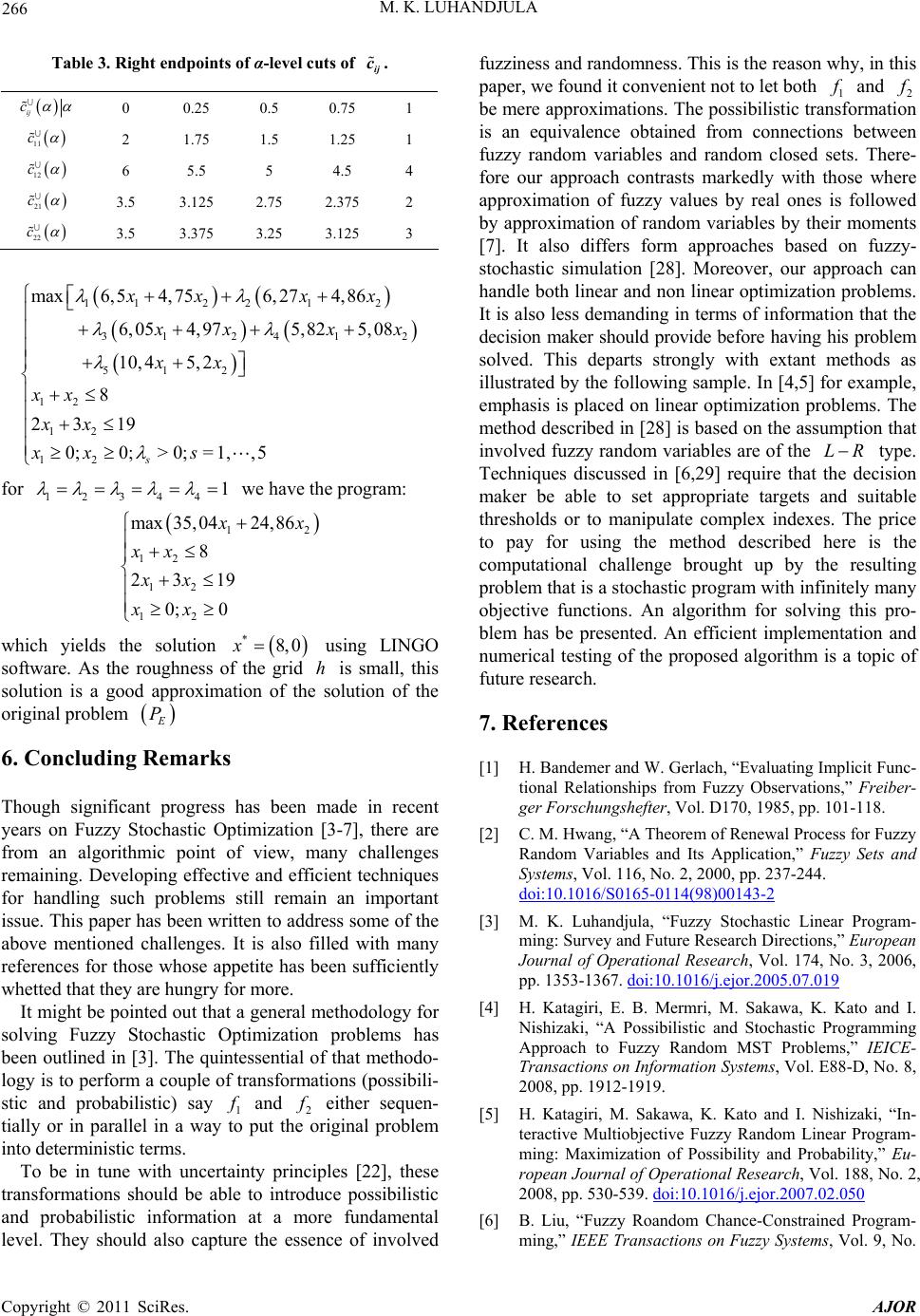

M. K. LUHANDJULA
266
Table 3. Right endpoints of α-level cuts of
ij
c.

ij
c



 0 0.25 0.5 0.75 1

11
c


 2 1.75 1.5 1.25 1

12
c


 6 5.5 5 4.5 4

21
c


 3.5 3.125 2.75 2.375 2

22
c


 3.5 3.375 3.25 3.125 3


1122 12
31 241
512
12
12
12
max6,5 4,756,274,86
5,0
,4
8
23
> 0,,5
s
xx xx


2


6,054,975,828
105,2
19
0;0;;=1
x
xx   x
for
x
xx
xx
xx



 














x
s
1243 4
1

      we have thrame prog:

12
max35,0424,86
12
12
12
19
0; 0
8
23
x
x 
x

x
xx
xx






which yields the solution LINGO
softwareth ughall, this
solution is a good approximn ohe
riginal problem

8,
*0x
the grid
atio the
using
is sm. As e roness ofh
n of solutiof t
o

E
P
6. Concluding Remarks
Though significant progress has been made in recent
years on Fuzzy Stochastic Optimization [3-7], there ae
from an algorithmic point of view, many challenges
remaining. Developing effective and efficient techniques
for handling such problems still remain an important
issue. This paper has been written to address some of the
e mentioned challenges. It
references for those whose appetite has been sufficiently
whetted that they are hungry for more.
It might be pointed out that a general mthodology for
solving Fuzzy Stochastic Optimization problems has
been outlined in [3]. The quintessential of that methodo-
logy is to perform a couple of transformations (possibili-
r
abov is also filled with many
e
stic and probabilistic) say 1
f
and 2
f
either sequen-
tially or in parallel in a way to put the original problem
into deterministic terms.
To be in tune uwith ncertainty principles [22], these
troduce possibilistic
at a more fundam
vel. They should also capture the essence of invo
transformations should be able to in
and probabilistic information ental
lved le
fuzziness and randomness. This is the reason why, in this
paper, we found it co nv enient not to let both 1
f
and 2
f
be mere approximations. The possibilistic transformation
is an equivalence obtained from connections between
fuzzy random variables and random closed sets. There-
fore our approach contrasts markedly with those where
approximation of fuzzy values by real ones is followed
by approximation of random variables by their moments
[7]. It also differs form approaches base fu
sto
y
ear optimization problems
m
d onzzy-
. The
chastic simulation [28]. Moreover, our approach can
handle both linear and non linear optimization problems.
It is also less demanding in terms of information that the
decision maker should provide before having his problem
solved. This departs stronglwith extant methods as
illustrated by the following sample. In [4,5] for example,
emphasis is placed on lin
ethod described in [28] is based on the assumption that
involved fuzzy random variables are of the LR

type.
Techniques discussed in [6,29] require that the decision
maker be able to set appropriate targets and suitable
thresholds or to manipulate complex indexes. The price
to pay for using the method described here is t
computational challenge brought up by the resulting
problem that is a stochastic program with infinitely many
objective functions. An algorithm for solving this pro-
blem has be presented. An efficient implementation and
numerical testing of the proposed algorithm is a topic of
future research.
7. References
[1] H. Bandemer and W. Gerlach, “Evaluating Implicit Func-
tional Relationships from Fuzzy Observations,” Freiber-
ger Forschungshefter, Vol. D170, 1985, pp. 101-118.
[2] C. M. Hwang, “A Theorem of Renewal Process for Fuzzy
Random Variables and Its Application,” Fuzzy Sets and
Systems, Vol. 116, No. 2, 2000, pp. 237-244.
doi:10.1016/S0165-0114(98)00143-2
he
[3] M. K. Luhandjula, “Fuzzy Stochastic Linear Program-
ming: Survey and Future Research Directions,” European
Journal of Operational Research, Vol. 174, No. 3, 2006,
pp. 1353-1367. doi:10.1016/j.ejor.2005.07.019
[4] H. Katagiri, E. B. Mermri, M. Sakawa, K. Kato and I.
Nishizaki, “A Possibilistic and Stochastic Programming
Approach to Fuzzy Random MST Problems,” IEICE-
Transactions on Information Systems, Vol. E88-D, No. 8,
2008, pp. 1912-1919.
[5] H. Katagiri, M. Sakawa, K. Kato and I. Nishizaki, “In-
teractive Multiobjective Fuzzy Random Linear Program-
ming: Maximization of Possibility and Probability,” Eu-
l of Operational Research, Vol. 188, No. 2,
539. doi:10.1016/j.ejor.2007.02.050
ropean Journa
2008, pp. 530-
[6] B. Liu, “Fuzzy Roandom Chance-Constrained Program-
ming,” IEEE Transactions on Fuzzy Systems, Vol. 9, No.

M. K. LUHANDJULA
267
5, 2001, pp. 713-720. doi:10.1109/91.963757
[7] Y. K. Liu and B. Liu, “A Class of Fuzzy Random Opti-
mization: Expected Value Models,” Information Sciences,
Vol. 155, No. 1-2, 2002, pp. 89-102.
doi:10.1016/S0020-0255(03)00079-3
[8] Y. K. Liu and B. Liu, “Fuzzy Random Programming with
Equilibrium Chance Constraints,” Information Sciences,
Vol. 170, No. 2-4, 2005, pp. 363-395.
doi:10.1016/j.ins.2004.03.010
[9] E. E. Ammar, “On Fuzzy Random Multiobjective Quad-
ratic Programming,” European Journal of Operational
Research, Vol. 193, No. 2, 2009, pp. 329-341.
doi:10.1016/j.ejor.2007.11.031
[10] Z. Zmeskel, “Value at Risk Methodology under Soft
Conditions Approach (Fuzzy-Stochastic Approach),” Eu-
ropean Journal of Operational Research, Vol. 161, No. 2,
2005, pp. 337-347. doi:10.1016/j.ejor.2003.08.048
[11] P. Dutta, D. Chakraborty and A. R. Roy, “A Single-Pe-
riod Inventory Model with Fuzzy Random Variable De-
mand,” Mathematical and Computer Modelling, Vol. 41,
No. 8-9, 2005, pp. 915-922.
doi:10.1016/j.mcm.2004.08.007
[12] F. Ben Abdelaziz, L. Enneifar and J. M. Martel, “A Mul-
tiobjective Fuzzy Stochastic Program for Water Resource
Optimization: The Case of Lake Management,” 2 005.
http://www.sharjah.ac.ae/academi/
[13] M. K. Luhandjula, “Optimization under Hybrid Uncer-
tainty,” Fuzzy Sets and Systems, Vol. 146, No. 2, 2004,
pp. 187-203. doi:10.1016/j.fss.2004.01.002
[14] C. Mohan and H. T. Nguyen, “An Interactive Satisfying
Method for Solving Multiobjective Mixed Fuzzy Sto-
chastic Programming Problems,” Fuzzy Sets and Systems,
Vol. 117, No. 1, 2001, pp. 61-79.
doi:10.1016/S0165-0114(98)00269-3
[15] S. Nanda, G. Panda and J. Dash, “A New Solution
Method for Fuzzy Chance Constrained Programming
Problem,” Fuzzy Optimization and Decision Making, Vol.
5, No. 4, 2006, pp. 355-370.
doi:10.1007/s10700-006-0018-8
[16] W. M. Kirby, “Paradigm Change in Operations Research:
Thirty Years of Debate,” Operations Research, Vol. 55,
No. 1, 2008, pp. 1-13. doi:10.1287/opre.1060.0310
[17] R. Kruze and K. D. Meyer, “Statistics with Vague Data,”
Reidel, Dordrecht, 1987. doi:10.1007/978-94-009-3943-1
[18] I. Moklanov, “Theory of Random Sets,” Springer, New
Sets and Systems: The-
Press, New York, 1980.
383-
York, 2005.
[19] G. Matheron, “Random Sets and Integral Geometry,”
John Wiley & Sons, New York, 1975.
[20] D. Dubois and H. Prade, “Fuzzy
ory and Applications,” Academic
[21] J. Bán, “Radon-Nikodyým Theorem and Conditional
Expectation of Fuzzy-Valued Measures and Variables,”
Fuzzy Sets and Systems, Vol. 34, No. 3, 1990, pp.
392. doi:10.1016/0165-0114(90)90223-S
[22] E. P. Klement, M. L. Puri and D. A. Ralescu, “Limit
Theorems for Fuzzy Random Variables,” Proceedings of
the Royal Society A, Vol. 407, No. 1832, 1986, pp. 171-
182. doi:10.1098/rspa.1986.0091
[23] C. X. Wu and M. Ma, “Embedding Problem of Fuzzy
Number Space,” Fuzzy Sets and Systems, Vol. 44, No. 1,
1991, pp. 33-38. doi:10.1016/0165-0114(91)90030-T
[24] H. C. Wu, “Evaluate Fuz zy Opt imiz at io n Problems Ba sed
on Biobjective Programming Problems,” Computer and
Mathematics with Applications, Vol. 47, No. 6-7, 2004,
pp. 893-902. doi:10.1016/S0898-1221(04)90073-9
[25] P. Kall, “Stochastic Linear Programming,” Springer, New
York. doi:10.1007/978-3-642-66252-2
[26] S. Vajda, “Probabilistic Programming,” Academic Press,
New York, 1972.
[27] G. J. Klir, “Principles of Uncertainty: What Are They?
Why Do We Need Them?” Fuzzy Sets and Systems, Vol.
74, No. 1, 1995, pp. 13-31.
doi:10.1016/0165-0114(95)00032-G
[28] J. Li, J. Xu and M. Gen, “A Class of Multiobjective Lin-
ear Programming Model with Fuzzy Random Coeffi-
cients,” Mathematical and Computer Modelling, Vol. 44,
No. 11-12, 2008, pp. 1097-1113.
doi:10.1016/j.mcm.2006.03.013
[29] V. H. Nguyen, “Solving Linear Programming Problems
under Fuzziness and Randomness Environment Using
Attainment Values,” Information Sciences, Vol. 177, No.
14, 2007, pp. 2971-2984.
doi:10.1016/j.ins.2007.01.032
[30] K. Glashoff and S. A. Gustafson, “Linear Optimization
and Approximation,” Springer-Verlag, Berlin, 1983.
doi:10.1007/978-1-4612-1142-6