J. Software Engineering & Applications, 2009, 2: 259-266
doi:10.4236/jsea.2009.24033 Published Online November 2009 (http://www.SciRP.org/journal/jsea)
259
Nonparametric Demand Forecasting with Right
Censored Observations
Bin ZHANG1,2 ; Zhongsheng HUA2
1Institute for Economics and Lingnan College, Sun Yat-sen University, Guangzhou, China; 2School of Management, University of
Science and Technology of China, Hefei, China.
Received July 17th, 2009; revised August 10th, 2009; accepted August 18th, 2009.
ABSTRACT
In a newsvendor inventory system, demand observations often get right censored when there are lost sales and no
backordering. Demands for newsvendor-type products are often forecasted from censored observations. The Kap-
lan-Meier product limit estimator is the well-known nonparametric method to deal with censored data, but it is unde-
fined beyond the la rgest observation if it is censored. To add ress this shortfall, some completion methods are suggested
in the literature. In th is paper, we propose two hypotheses to investigate estimation bia s of the product limit estimator,
and provide three modified completion methods based on the proposed hypotheses. The proposed hypotheses are veri-
fied and the proposed completion methods are compared with current nonparametric completion methods by simulation
studies. Simulation results show that biases of the proposed completion methods are significantly smaller than that of
those in the literatu re.
Keywords: Forecasting, Demand, Censored, Nonparametric, Product Limit Estimator
1. Introduction
In a newsvendor inventory system, a decision maker
places an order before the selling season with stochastic
demand. If too much is ordered, stock is left over at the
end of the period, whereas if too little is ordered, sales
are lost. The optimal order quantity is often set based on
the well-known critical ratio [1], therefore demand ob-
servations often get right censored when there are lost
sales and no backordering. Because lost sales cannot be
observed, the available sales data actually reflect the
stock available for sale, rather than the true demand.
Demands for newsvendor-type products are often fore-
casted from censored observations.
The problem of demand forecasting in the presence of
stockouts is a well-known problem of handling censored
observations, which was recognized by [2]. Approaches
of handling censored observations can be divided into
two classes: (1) parametric method, which often assumes
that the observations come from specific theoretical dis-
tribution and then estimate parameters of the assumed
distribution by applying maximum likelihood estimation
or some updating procedures [3]; This method is often
used in density forecasting [4]; (2) nonparametric method,
which is often established based on the product limit es-
timator [5], and attempts to address the problem of the
“undefined region” beyond the largest observation when
it is censored [6].
Parametric methods for demand forecasting from cen-
sored observations have been investigated in [7−14].
These works have been briefly reviewed in [15], and it
has been indicated in [15] that it is difficult to determine
the shape or family of demand distribution in advance
when demand observations are censored.
The product limit (PL) estimator is a nonparametric
maximum likelihood estimator of a distribution function
based on censored data. If the largest observation is cen-
sored, the PL estimator is developed to estimate the
left-hand side of demand distribution, but it is undefined
for the right-hand side of distribution function. Under the
assumption that there are more information besides the
censored observations, Lau and Lau [3] and Zhang et al.
[15] have investigated the problems of estimating the
right-hand side of demand distributions.
Without additional information besides the censored
observations, truncation techniques or completion meth-
ods are usually employed to define the whole distribution
function. Truncation techniques are based on the
data-driving rules, which include two common truncation
rules: (1) truncating at the largest observation if it is
censored, and (2) truncating at (n−l)th order statistics [6].
These truncation rules may intuitively appear to have
good properties by avoiding problems in tail, but they
will incur large bias because the location of the ignored

Nonparametric Demand Forecasting with Right Censored Observations 260
region is a random event. Completion methods aim to
redefine the PL estimator beyond the largest observation
if it is censored. We will briefly review nonparametric
completion methods in the next section.
In this paper, we propose two hypotheses to investi-
gate estimation bias of the PL estimator, and provide
three modified completion methods based on the pro-
posed hypotheses. The proposed hypotheses are verified
and the proposed completion methods are compared with
current nonparametric completion methods in the litera-
ture by simulation studies.
The remainder of this paper is structured as follows.
We briefly introduce the PL estimator and review current
nonparametric completion methods suggested in the lit-
erature. Then we propose two hypotheses to investigate
estimation bias of the PL estimator, and provide three
modified completion methods. We further verify the two
hypotheses and compare the proposed completion meth-
ods with current nonparametric completion methods by
simulation studies. The paper ends with some concluding
remarks.
2. Nonparametric Completion Methods
In this section, we first introduce the PL estimator in the
context of an inventory system, and then we review cur-
rent nonparametric completion methods for the PL esti-
mator suggested in the literature.
2.1 Product Limit Estimator
Let i
X
, , be iid (independent identi-
cally-distributed) demand from distribution F, and in-
ventory level , be iid from distribution
G. It is often to assume that both F and G are continuous
and defined on the interval . In an inventory sys-
tem, demand
1, 2,,i
i
Y1, 2i
i
n
n, ,

0,


X
is censored on the right by the avail-
able inventory level , and we observe
i
Yi
Z



min ,
i
XY
ii
and

ii
I
XY  , , where 1, 2,,in

I
 stands for the indicator function, and i

indicates
whether demand observation i
Z
is censored (0
i


) or
not (1
i

).
Kaplan and Meier [5] introduced the PL estimator for
the survival function , which is esti-
mated as follows:
 
1St Ft


:
:
1
ˆ11
in
I
Zt
nin
i
St ni




 



(1)
where :in
Z
denotes the ith ordered observation
among all i
Z
, and :in

corresponds to :in
Z
. From the
above definition, it is observed that the PL estimator is
undefined beyond the largest observation, i.e., for
and
:nn
tZ:0
nn


.
2.2 Review of Current Completion Methods
To overcome the shortfall of the PL estimator that it is
undefined beyond the largest observation, some comple-
tion methods are suggested in the literature. Efron [16]
introduced the notion of self-consistency, i.e.,


ˆE
St 0

, for . (2)
:nn
tZ
Gill [17] defined the survival function by
 

:
:
:1
ˆ11
1
in
I
Zt
in
i
ni



 



n
Gn
n




St

for (3)
:nn
tZ
Chen and Phadia [18] modified it as


:
1:
:1
11
1
in
I
ˆ
Zt
in
ni
cni





 



n
Cn
 St for(4)
:nn
tZ
where


0, 1


2
Ftd

c
ˆ
E
 is determined by minimizing the mean
squared error loss
 


2
00
ˆ
FtFtEStSt dSt



(5)
Clearly, the extreme values of scalar c yield Efron’s and
Gill’s versions, respectively.
Besides the above three constant completion methods,
there are two curve completion methods suggested in the
literature. Brown et al [19] suggested an exponential
completion method as follows:


ˆ
B
t
e
B
St


, for . (6)
:nn
tZ
The parameter
B

is set by solving

:
:
ˆ
B
nn
Z
nn
SZ e
  ,
where


:nn nn
Z
:
0, 0
limZ





. Let ()i
Z
, , de-
note the m ordered uncensored demand observations, the
remaining
1,im
nm

observations are censored ones.
Moeschberger and Klein [20] attempted to complete


ˆ
St by a two-parameter Weibull function as follows:

ˆM
Stk
Mt
e
 , for (7)
:nn
tZ
The two parameters
M

and k in Equation (7) are de-
termined by solving




k
Mm
t
m
SZ e
 

ˆ and





1
k
Mm
t
e



1
ˆm
SZ.
When a completion method is used, the bias of


ˆ
St,








ˆ
B
t EStSt
, is entirely determined by the
completion method [21]. For a completion method, it is
clear that the “undefined region” has the most contribu-
tion to the bias of the PL estimator. One might think that
this region could be in some sense ignored, as it is sug-

Nonparametric Demand Forecasting with Right Censored Observations 261
gested in truncation techniques. Because the location of
this region is a random event, simply ignoring the “unde-
fined region” will result in a large bias [6].
The bias of is negative and asymptotically
zero as , whereas the bias of

ˆE
St
t


ˆG
St
ˆC
S
t

St
is positive
and increasing as . The bias using any other
completion method will be bounded by the biases of
and [6]. The bias of changes
from negative to positive and it is increasing as .
If an estimator is asymptotically zero as , we say
that it has completeness, which is necessary for estimat-
ing moments of distribution. ,
t

t


ˆE
St ˆG S

t
t
ˆE


t
ˆB
S, and


ˆM
St

ˆB
St
have completeness since they are asymptotically
zero as t, whereas and do not
have the completeness. The curve completion methods,
, and


t
ˆG
S

t
ˆC
S


ˆM
St

ˆE
St
satisfy the downward sloping
monotonicity of survival function, but the constant com-
pletion methods, ,



ˆG
St and do not.

ˆC
St
3. New Completion Methods
In this section, we first propose two hypotheses to inves-
tigate estimation bias of the PL estimator at two special
points, and provide three modified completion methods
based on the proposed hypotheses. Then we simplify
show the nonparametric completion methods by an ex-
ample.
3.1 Estimation Bias of the PL Estimator
If demand observations i
X
, , are observ-
able, then its empirical survival function
1, 2,,i n


St can be
expressed as follows:
 
1
1
1
n
i
i
StIX t
n
 


:
(8)
Since :nn nn
X
Z , the value of

St at point :nn
Z

can
be rewritten as
 
 ::
::
1
1
1
1
1
1
11
in nn
n
nni nn
i
IX Z
n
i
SZIX Z
n
ni






 

 






(9)
According to Equation (1), the estimation value of the PL
estimator at point :nn
Z
 is

1
1:
:1
ˆ11
nin
nn i
SZ ni




 





(10)
To compare

:nn
SZ


1
1
:1
1
11
n
nn i
SZ ni



 





(11)
From Equations (9–11), can be viewed as a
modification of

:
ˆnn
SZ



:nn
SZ
 by replacing
by 1 (from Equation (9–11)), and then replacing 1 by

::in nn
IX Z


:in

(from Equation (11,10)). By introducing these two
replacements, it is clear that



::nn nn
SZ

SZ

and




:
ˆ
nn nn
SZ

:


SZ
. This indicates that will
underestimate

:nn
SZ




:nn
SZ
, will overestimate

:
ˆnn
SZ




:nn

SZ
, but


:
ˆnn
SZ
 will underestimate or overesti-
mate


:nn
SZ
.
The sign of bias


:
ˆnn nn
SZ SZ



:

is completely de-
termined by


::in nn
IX Z

 and :in

, .
Since
1, 2,,1in


::nn
Z


in
IX and :in

are random variables
determined by i
X
and , , the bias is
also a random variable and its sign also depends on
i
Y1, 2,i,n
i

X
and ,
i
Y1, 2,,in

. In the case when 1: :nn nn
X
Z


is satisfied and there is at least one censored observation
among :in
Z
, 1, 2,,1in

, must overesti-
mate

:nn
SZ


ˆ


:nn
SZ
. We argue that :in

has more important
influence on the estimation bias than
does, i.e., the PL estimator will statistically overestimate
at point

::in nn
IX Z


:nn
Z

. Based on this perception, we present the
following hypothesis:
Hypothesis 1:
Denote by




::
ˆ
nnnn nn
BZSZ SZ



:

, then


:nn
BZ

is statistically larger than zero.
Since the PL estimator is a piecewise right continuous
function, and the largest uncensored observation

m
Z
is
a right continuous piecewise point, so the relative esti-
mation bias of the PL estimator at point

m
Z
should be
statistically smaller than that at point :nn
Z
. That is, the
PL estimator statistically provide more accurate estima-
tion at point

m
Z
than at :nn
Z
. Therefore, we have the
following hypothesis:
Hypothesis 2:
Denote by



 
ˆ
RtStStSt , then



m
RZ is
statistically smaller than


:nn
RZ
 
and , we introduce

:
ˆnn
SZ
.

Nonparametric Demand Forecasting with Right Censored Observations 262
34, 34, 37*, 38, 44*, 45*, 47*, 50, 50, 50, 60, 60*, 65* (8
times), where asterisk indicates a censored observation,
e.g., the third entry ‘37*’ means that was ob-
served on a day when
337Z
337Y

, implying that .
337X
3.2 Modified Completion Methods
In the spirit of the exponential curve completion method
suggested by [19], we provide three modified completion
methods based on the proposed hypotheses.
For this example, the various aforementioned comple-
tion methods are plotted in Figure 1. From Figure 1 it can
be observed that, the five curve completion methods sat-
isfy the downward sloping monotonicity of survival
function, and that the five curve completion methods and
Efron’s self-consistent completion have the complete-
ness.
Hypothesis 1 implies that the PL estimator will statis-
tically overestimate at point :nn
Z

. Therefore bias can be
reduced if parameter of the exponential curve is set by solv-
ing

:
:
ˆ
D
nn
Z
nn
dSZ e
 

 instead of

:
:
ˆ
B
nn
Z
nn
SZ e
  ,
where


0,1d is an adjusted factor for overcoming
the overestimation of the PL estimator at point :nn
Z

.
Chen and Phadia [18] proposed an optimal constant
completion by setting . Similarly, we
set . This parameter setting is presented
because scalar d should not be larger than one in solving

:
ˆ
nn 

:
ˆ
nn
Z

SZ

min2 ,1dc
cS
D

.
4. Simulation Studies
In this section, we verify the two proposed hypotheses
and compare the aforementioned completion methods by
simulation studies.
4.1 Simulation Experiments
In our simulation studies, we design two experiments
under an inventory system with some specific distribu-
tions as follows:
Hypothesis 2 indicates that the relative estimation bias
of the PL estimator at point
 m
Z
is statistically smaller
than that at point :nn
Z
. Therefore bias can be reduced if
parameter of the exponential curve is set by solving
instead of



ˆLm
Z
m
SZ e
 


:
:
ˆ
B
nn
Z
nn
SZ e
 


. Since
the exponential curve may approximately pass the two
points and

ˆ
,
m
ZS



m
Z



::
ˆ
, nn ZdSZ


nn , the pa-
rameter of the exponential curve can also be set as

2
ALD
  .
Experiment 1: Following [22−23], we take demand
distribution F to be a Weibull distribution,




1exp a
F
xx for with a=1 and 2. To
reflect a variety of censoring distribution patterns, we
also follow [23] to take Weibull distribution,
0x


Gy


1exp b uy




for with 0x2ba, ba

, and
2ba

, as our censoring inventory distribution. This
gives the hazard rate


bb
ut a ht , which is decreasing
for 1ba

, constant for 1ba, and increasing
1ba. The scale factor u in is adjusted in such
a way so that the expected stockout probability (ESP)

Gy

3.3 An Illustrative Example
In a case study of a newsvendor inventory system, Lau
and Lau [3] presented 20 ordered daily sales observations:
Figure 1. Comparison of the eight completion methods for the PL estimator

Nonparametric Demand Forecasting with Right Censored Observations 263
Table 1. Statistical results of


:nn
BZ
 in Experiment 1
b/a =0.5 b/a =1 b/a =2
a=1 a=2 a=1 a=2 a=1 a=2
Mean of

:nn
BZ
0.0082 0.0102 0.0269 0.0259 0.0300 0.0312
Std. Dev. of

:nn
BZ
0.0667 0.0681 0.1075 0.1098 0.1487 0.1511
Lower 0.0041 0.0060 0.0202 0.0191 0.0208 0.0218
95% C.I. of


:nn
BZ

Upper 0.01230.01450.0335 0.03270.0392 0.0406
Table 2. Statistical results of


:nn
BZ
 in Experiment 2
ESP =1/3 ESP =1/2 ESP =2/3
1


2


1


2


1

 2


Mean of


:nn
BZ
 0.0758 0.0893 0.1637 0.1839 0.2758 0.3144
Std. Dev. of

:nn
BZ
0.0607 0.0705 0.1053 0.1181 0.1419 0.1464
Lower 0.07200.0849 0.1572 0.1766 0.2670 0.3053
95% C.I. of

:nn
BZ

Upper 0.0796 0.0936 0.1703 0.1912 0.2846 0.3235
is 1/3, 1/2, or 2/3. These values thus completely specify
the hazard rate. The reader is referred to [23] for further
details. This experiment is applied for investigating the
case when hazard rate is decreasing, constant or increas-
ing.
Experiment 2: Analogous to [8], we express the rela-
tion between demand X and sales Z by writing sales as a
random proportion of demand, i.e., iii
Z
WX
1
i
W
, where
is a random variable taking values on the interval
[0.5,1]. For periods with no stockout, , and there-
fore sales and demand are equal; for periods in which a
stockout has occurred, sales will be less than demand
with . We assume that stockouts occur in each
period (independently) with probability ESP and when a
stockout occurs, sales
i
W
1
i
W
i
Z
is a random (uniformly dis-
tributed) proportion of demand i
X
. In our case studies,
we take F to be a lognormal distribution with location
parameter 4, and shape parameter 1

 and 2, and we
also set ESP=1/3, 1/2, and 2/3. This experiment is de-
signed for investigating the case when hazard rate
changes from increasing to decreasing.
In the above two experiments, we have four different
cases in terms of hazard rate: decreasing, constant, in-
creasing, and changing from increasing to decreasing. In
comparison with Experiment 1, Experiment 2 makes an
additional assumption on the relation between demand
and sales, i.e., sales is a random (uniformly distributed)
proportion of demand.
Considering the combination of the parameters in the
above two experiments, under each of four cases of haz-
ard rate, we have 6 different combinations of the pa-
rameters. Under each parameters’ combination, we set
the number of observations n=20, and randomly generate
1000 simulation runs. To ensure the applicability of the
completion method suggested by Moeschberger and
Klein [20], the number of uncensored observations in
each simulation run is restricted to be larger than 3. For
the convenience of comparison, the largest observation in
each simulation run is restricted to be a censored one.
4.2 Hypotheses Verification
Under each of four cases of hazard rate, we calculate


:nn
BZ
 under 1000 simulation runs for verifying Hy-
pothesis 1. Statistical results of


:nn
BZ
 are reported in
Tables 1 and 2. In these tables, 95% C.I. is short for 95%
confidence level.
Results shown in Tables 1 and 2 verify Hypothesis 1,
i.e., the PL estimator statistically overestimates at point
:nn
Z

. Table 1 also illustrates that increases
with the increase of b/a, this implies that the estimation
bias of the case with increasing hazard rate is larger than
that of the case with decreasing hazard case. Table 2 also
illustrates that

:nn
BZ




:nn
BZ
 increases as the expected
stockout probability increases.
To verify the correctness of Hypothesis 2, we calculate


:nn
RZ
 and



m
RZ under each of four cases of hazard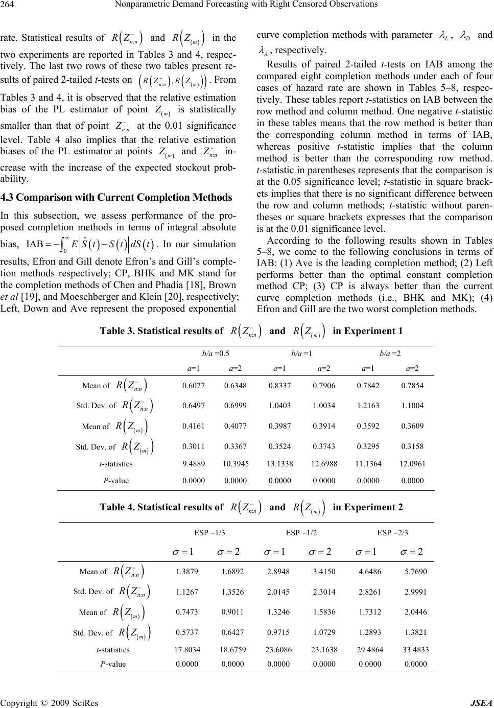

Nonparametric Demand Forecasting with Right Censored Observations 264
rate. Statistical results of


:nn
RZ
 and in the
two experiments are reported in Tables 3 and 4, respec-
tively. The last two rows of these two tables present re-
sults of paired 2-tailed t-tests on


m
RZ








:nn
RZ


m
,m RZ

. From
Tables 3 and 4, it is observed that the relative estimation
bias of the PL estimator of point
Z
is statistically
smaller than that of point :nn
Z

at the 0.01 significance
level. Table 4 also implies that the relative estimation
biases of the PL estimator at points

m
Z
and :nn
Z

in-
crease with the increase of the expected stockout prob-
ability.
4.3 Comparison with Current Completion Methods
In this subsection, we assess performance of the pro-
posed completion methods in terms of integral absolute
bias,
 
dS t
0
ˆ
IAB ES t

 
S t. In our simulation
results, Efron and Gill denote Efron’s and Gill’s comple-
tion methods respectively; CP, BHK and MK stand for
the completion methods of Chen and Phadia [18], Brown
et al [19], and Moeschberger and Klein [20], respectively;
Left, Down and Ave represent the proposed exponential
curve completion methods with parameter
L

,
D

and
A

, respectively.
Results of paired 2-tailed t-tests on IAB among the
compared eight completion methods under each of four
cases of hazard rate are shown in Tables 5–8, respec-
tively. These tables report t-statistics on IAB between the
row method and column method. One negative t-statistic
in these tables means that the row method is better than
the corresponding column method in terms of IAB,
whereas positive t-statistic implies that the column
method is better than the corresponding row method.
t-statistic in parentheses represents that the comparison is
at the 0.05 significance level; t-statistic in square brack-
ets implies that there is no significant difference between
the row and column methods; t-statistic without paren-
theses or square brackets expresses that the comparison
is at the 0.01 significance level.
According to the following results shown in Tables
5–8, we come to the following conclusions in terms of
IAB: (1) Ave is the leading completion method; (2) Left
performs better than the optimal constant completion
method CP; (3) CP is always better than the current
curve completion methods (i.e., BHK and MK); (4)
Efron and Gill are the two worst completion methods.
Table 3. Statistical results of


:nn
RZ
 and



m
RZ in Experiment 1
b/a =0.5 b/a =1 b/a =2
a=1 a=2 a=1 a=2 a=1 a=2
Mean of


:nn

RZ 0.6077 0.6348 0.8337 0.7906 0.7842 0.7854
Std. Dev. of


:nn


RZ 0.6497 0.6999 1.0403 1.0034 1.2163 1.1004
Mean of


m

RZ 0.4161 0.4077 0.3987 0.3914 0.3592 0.3609
Std. Dev. of


m
RZ 0.3011 0.3367 0.3524 0.3743 0.3295 0.3158
t-statistics 9.4889 10.3945 13.1338 12.6988 11.1364 12.0961
P-value 0.0000 0.0000 0.0000 0.0000 0.0000 0.0000
Table 4. Statistical results of


:nn
RZ
 and



m
RZ in Experiment 2
ESP =1/3 ESP =1/2 ESP =2/3
1

 2


1


2


1


2


Mean of


:nn

RZ 1.38791.68922.89483.41504.6486 5.7690
Std. Dev. of


:nn



m

RZ
RZ
1.12671.35262.01452.30142.8261 2.9991
Mean of 0.74730.90111.32461.58361.7312 2.0446
Std. Dev. of


m
RZ 0.57370.64270.97151.07291.2893 1.3821
t-statistics 17.803418.675923.608623.163829.4864 33.4833
P-value 0.00000.00000.00000.00000.0000 0.0000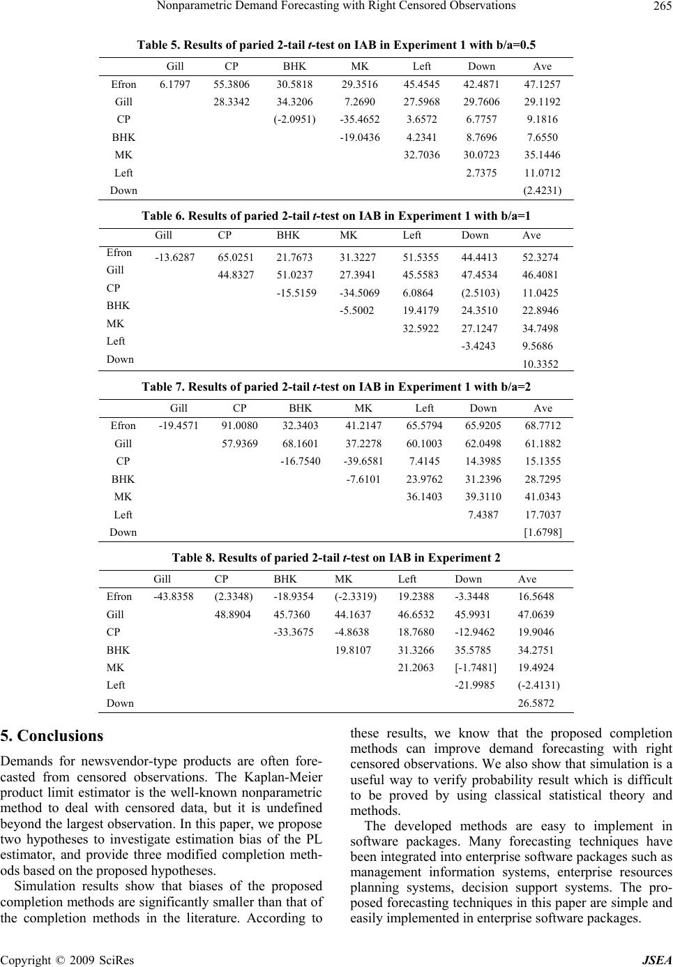

Nonparametric Demand Forecasting with Right Censored Observations 265
Table 5. Results of paried 2-tail t-test on IAB in Experiment 1 with b/a=0.5
Gill CP BHK MK Left Down Ave
Efron 6.1797 55.3806 30.5818 29.3516 45.4545 42.4871 47.1257
Gill 28.3342 34.3206 7.2690 27.5968 29.7606 29.1192
CP (-2.0951) -35.4652 3.6572 6.7757 9.1816
BHK -19.0436 4.2341 8.7696 7.6550
MK 32.7036 30.0723 35.1446
Left 2.7375 11.0712
Down (2.4231)
Table 6. Results of paried 2-tail t-test on IAB in Experiment 1 with b/a=1
Gill CP BHK MK Left Down Ave
Efron -13.6287 65.0251 21.7673 31.3227 51.5355 44.4413 52.3274
Gill 44.8327 51.0237 27.3941 45.5583 47.4534 46.4081
CP -15.5159 -34.5069 6.0864 (2.5103) 11.0425
BHK -5.5002 19.4179 24.3510 22.8946
MK 32.5922 27.1247 34.7498
Left -3.4243 9.5686
Down 10.3352
Table 7. Results of paried 2-tail t-test on IAB in Experiment 1 with b/a=2
Gill CP BHK MK Left Down Ave
Efron -19.4571 91.0080 32.3403 41.2147 65.5794 65.9205 68.7712
Gill 57.9369 68.1601 37.2278 60.1003 62.0498 61.1882
CP -16.7540 -39.6581 7.4145 14.3985 15.1355
BHK -7.6101 23.9762 31.2396 28.7295
MK 36.1403 39.3110 41.0343
Left 7.4387 17.7037
Down [1.6798]
Table 8. Results of paried 2-tail t-test on IAB in Experiment 2
Gill CP BHK MK Left Down Ave
Efron -43.8358 (2.3348) -18.9354 (-2.3319) 19.2388 -3.3448 16.5648
Gill 48.8904 45.7360 44.1637 46.6532 45.9931 47.0639
CP -33.3675 -4.8638 18.7680 -12.9462 19.9046
BHK 19.8107 31.3266 35.5785 34.2751
MK 21.2063 [-1.7481] 19.4924
Left -21.9985 (-2.4131)
Down 26.5872
5. Conclusions
Demands for newsvendor-type products are often fore-
casted from censored observations. The Kaplan-Meier
product limit estimator is the well-known nonparametric
method to deal with censored data, but it is undefined
beyond the largest observation. In this paper, we propose
two hypotheses to investigate estimation bias of the PL
estimator, and provide three modified completion meth-
ods based on the proposed hypotheses.
Simulation results show that biases of the proposed
completion methods are significantly smaller than that of
the completion methods in the literature. According to
these results, we know that the proposed completion
methods can improve demand forecasting with right
censored observations. We also show that simulation is a
useful way to verify probability result which is difficult
to be proved by using classical statistical theory and
methods.
The developed methods are easy to implement in
software packages. Many forecasting techniques have
been integrated into enterprise software packages such as
management information systems, enterprise resources
planning systems, decision support systems. The pro-
posed forecasting techniques in this paper are simple and
easily implemented in enterprise software packages.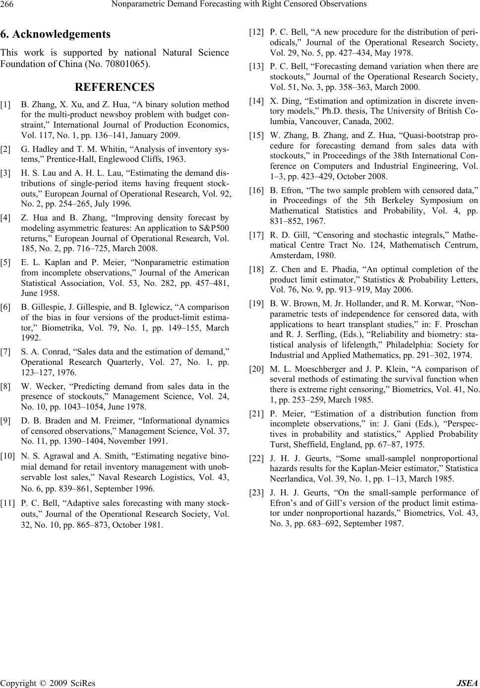

Nonparametric Demand Forecasting with Right Censored Observations 266
6. Acknowledgements
This work is supported by national Natural Science
Foundation of China (No. 70801065).
REFERENCES
[1] B. Zhang, X. Xu, and Z. Hua, “A binary solution method
for the multi-product newsboy problem with budget con-
straint,” International Journal of Production Economics,
Vol. 117, No. 1, pp. 136–141, January 2009.
[2] G. Hadley and T. M. Whitin, “Analysis of inventory sys-
tems,” Prentice-Hall, Englewood Cliffs, 1963.
[3] H. S. Lau and A. H. L. Lau, “Estimating the demand dis-
tributions of single-period items having frequent stock-
outs,” European Journal of Operational Research, Vol. 92,
No. 2, pp. 254–265, July 1996.
[4] Z. Hua and B. Zhang, “Improving density forecast by
modeling asymmetric features: An application to S&P500
returns,” European Journal of Operational Research, Vol.
185, No. 2, pp. 716–725, March 2008.
[5] E. L. Kaplan and P. Meier, “Nonparametric estimation
from incomplete observations,” Journal of the American
Statistical Association, Vol. 53, No. 282, pp. 457–481,
June 1958.
[6] B. Gillespie, J. Gillespie, and B. Iglewicz, “A comparison
of the bias in four versions of the product-limit estima-
tor,” Biometrika, Vol. 79, No. 1, pp. 149–155, March
1992.
[7] S. A. Conrad, “Sales data and the estimation of demand,”
Operational Research Quarterly, Vol. 27, No. 1, pp.
123–127, 1976.
[8] W. Wecker, “Predicting demand from sales data in the
presence of stockouts,” Management Science, Vol. 24,
No. 10, pp. 1043–1054, June 1978.
[9] D. B. Braden and M. Freimer, “Informational dynamics
of censored observations,” Management Science, Vol. 37,
No. 11, pp. 1390–1404, November 1991.
[10] N. S. Agrawal and A. Smith, “Estimating negative bino-
mial demand for retail inventory management with unob-
servable lost sales,” Naval Research Logistics, Vol. 43,
No. 6, pp. 839–861, September 1996.
[11] P. C. Bell, “Adaptive sales forecasting with many stock-
outs,” Journal of the Operational Research Society, Vol.
32, No. 10, pp. 865–873, October 1981.
[12] P. C. Bell, “A new procedure for the distribution of peri-
odicals,” Journal of the Operational Research Society,
Vol. 29, No. 5, pp. 427–434, May 1978.
[13] P. C. Bell, “Forecasting demand variation when there are
stockouts,” Journal of the Operational Research Society,
Vol. 51, No. 3, pp. 358–363, March 2000.
[14] X. Ding, “Estimation and optimization in discrete inven-
tory models,” Ph.D. thesis, The University of British Co-
lumbia, Vancouver, Canada, 2002.
[15] W. Zhang, B. Zhang, and Z. Hua, “Quasi-bootstrap pro-
cedure for forecasting demand from sales data with
stockouts,” in Proceedings of the 38th International Con-
ference on Computers and Industrial Engineering, Vol.
1–3, pp. 423–429, October 2008.
[16] B. Efron, “The two sample problem with censored data,”
in Proceedings of the 5th Berkeley Symposium on
Mathematical Statistics and Probability, Vol. 4, pp.
831–852, 1967.
[17] R. D. Gill, “Censoring and stochastic integrals,” Mathe-
matical Centre Tract No. 124, Mathematisch Centrum,
Amsterdam, 1980.
[18] Z. Chen and E. Phadia, “An optimal completion of the
product limit estimator,” Statistics & Probability Letters,
Vol. 76, No. 9, pp. 913–919, May 2006.
[19] B. W. Brown, M. Jr. Hollander, and R. M. Korwar, “Non-
parametric tests of independence for censored data, with
applications to heart transplant studies,” in: F. Proschan
and R. J. Serfling, (Eds.), “Reliability and biometry: sta-
tistical analysis of lifelength,” Philadelphia: Society for
Industrial and Applied Mathematics, pp. 291–302, 1974.
[20] M. L. Moeschberger and J. P. Klein, “A comparison of
several methods of estimating the survival function when
there is extreme right censoring,” Biometrics, Vol. 41, No.
1, pp. 253–259, March 1985.
[21] P. Meier, “Estimation of a distribution function from
incomplete observations,” in: J. Gani (Eds.), “Perspec-
tives in probability and statistics,” Applied Probability
Turst, Sheffield, England, pp. 67–87, 1975.
[22] J. H. J. Geurts, “Some small-samplel nonproportional
hazards results for the Kaplan-Meier estimator,” Statistica
Neerlandica, Vol. 39, No. 1, pp. 1–13, March 1985.
[23] J. H. J. Geurts, “On the small-sample performance of
Efron’s and of Gill’s version of the product limit estima-
tor under nonproportional hazards,” Biometrics, Vol. 43,
No. 3, pp. 683–692, September 1987.