Journal of Computer and Communications
Vol.06 No.11(2018), Article ID:88549,12 pages
10.4236/jcc.2018.611012
Main Processes for OVS-1A & OVS-1B: From Manufacturer to User
Shixiang Cao, Wenwen Qi, Wei Tan, Nan Zhou, Yongfu Hu
Satellite Technique Support Team, Beijing Institute of Space Mechanics & Electricity, Beijing, China


Received: October 16, 2018; Accepted: November 12, 2018; Published: November 19, 2018
ABSTRACT
Commercial remote sensing has boosted a new revolution in traditional processing chain. During the development of OVS-1A and OVS-1B, we construct the main processing pipeline for ground and calibration system. Since these two satellites utilize colorful video imaging pattern, the underlying video stabilization and color adjustment is vital for end user. Besides that, a full explanation is given for researchers to shed light on how to promote the imagery quality from manufacturing satellite camera to generate video products. From processing system, the demo cases demonstrate its potential to satisfy end user. Our team also releases the possible improvement for video imaging satellite in the coming future.
Keywords:
Remote Sensing, Video Satellite, Image Processing, Manufacture Improvement

1. Introduction
The OVS-1A and OVS-1B video satellites (also known as ZHUHAI-1 01 and ZHUHAI-1 02 [1]) were launched on June 15, 2017, and the two equipped cameras can capture 10-bit image or 8-bit video sequence at 20 fps both converting from Bayer formatted data.
After one year running around, we feel honorable to reveal the main processing methods used, which may be different from general close range community, for end user.
In the past few years, mini satellite for commercial user is largely developed from overhead video imaging which can be recently dated back to typical SkySat [2]. Nowadays, the surveillance need for local interesting event is boosted in many industrial or military applications, such as interesting region surveillance, coastline defense [3].
Given a tight budget, Beijing Institute of Space Mechanics & Electricity (shown as BISME hereinafter) undertook the contract in 2016 from Zhuhai Orbita Aerospace Science & Technology Co, Ltd. (available at http://www.myorbita.net/), which must be finished in one year. Our engineers inherit some effective design from industrial applications and furthermore proposed some techniques to promote higher quality for standard product.
Figure 1 and Table 1 show the appearance and system characteristics of these two satellite cameras. Opposite to the combined imaging plane of SkySat, the platform chooses to rotate to hold the nadir viewport all the time, and a common 90 seconds duration video sequences are stored on board or directly transferred to ground station.

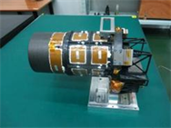


Figure 1. Camera in lab and Imaging mode: (Top left) OVS-1A; (Top right) OVS-1B; (Bottom left) video sequences; (Bottom right) multi footprint to get large region.

Table 1. Camera system charactersitic.
From the working mode in Figure 1, one thing should be noted the viewing angle always varies, and bad effect also comes from the platform vibration at 550 km, even its absolute value is small, this is why we carefully designed the stabilization method.
To the radiometric calibration, a classical and uniform region is not practical any more [4], and statistical analysis for line sensor fails the area plane detector, and the real value of each pixel should be computed individually.
A subset of real image covering Cape Town is given in Figure 2. As a first impression, we list all the techniques embedded in this paper:
1) How to get high level radiometric calibration result for area device;
2) How to make change for Bayer formatted pixel to get an uniform image;
3) How to calculate the color transformation for true RGB;
4) How to implement video stabilization and approximately still video;
5) Geometrical processes for video sequences.
2. Radiometric Model
Before going to the main process, the linear model should be given for imaging pixel, and the reader can go to this section after knowing the challenge for future devices. The widely used is linear model [5] [6]: the DN value can be calibrated as a linear relationship with radiance.
Suppose the area scanner contains pixels, in this paper, digital number of any pixel in image B can be expressed as:
, , (1)
(2)

Figure 2. Raw image from OVS-1A covering Cape Town. Please zoom the electric version to see the mosaic phenomenon (Bayer format). Image is linearly stretched into [0-255] for visualization.
where ―the DN value in image B;
―equivalent radiance from calibration light;
―gain for radiance;
―offset for radiance;
―relative spectral response;
―transmittance of optical system;
and ―range of wave length.
In most cases, the non-uniform noise in image mainly comes from the gain and offset differences of every pixel.
3. Main Processing
From the calibration images, the normal no-uniformity coefficient can be calculated. Then stack the surface image at high and low digital value to generate two virtual images, a linear fitness of these two images modifies the initial NU coefficients. After that, we utilize the radiometric parameter to enhance image, generate L1 to L2 and video product. Figure 3 shows the main pipeline of following steps.
3.1. No-Uniformity Correction
Using the initial calibration data, the top of atmospheric no-uniformity coefficient for raw data can be drawn as:
(3)
(4)

Figure 3. Main processing chart of processing method.
(5)
(6)
Above processes fit response of every pixel to the statistical mean value, and generate the initial gain and offset coefficients and . Figure 4 shows the correction result in lab.
Specially, for Bayer image, there should be two normal approaches for RGB channels calibration separately:
1) interpolate Bayer to virtual RGB, calibrate RGB separately;
2) pick real RGB from Bayer, calibrate them and demosaic to get final result.
We found the latter one is a physical and strict data reconstruction method which generates better result. In one word, Bayer image cannot be interpolated to RGB before radiometric calibration. Figure 5 illustrates the specific operation.


Figure 4. Radiometric correction in lab: (left) input image; (right) output result.

Figure 5. Pick out physically imaging pixel and reconstruct RGB image.
After the launch, non-uniform noise still residues in real image, and it can be easily attributed to atmosphere or some other transfer jitter. Actually, with the help of our former work [7], we stacked the high DN image from mid latitude cloud and low level image covering nightly ocean, and got near 3% radiometric result after a second calibration. Figure 6 outlines the strengthened result from our method.
3.2. Color Adjustment and Image Dehaze
Excellent results can usually be achieved with the inexpensive, widely-available 24-patch X-Rite color checker. The CCM (color correction matrix) can be applied to images to achieve optimum color reproduction, which is defined as the minimum mean squared color error between a corrected test chart patches and the corresponding reference values, which can be the standard (published) values.
From the radiometric model, the R, G, and B values of each output (corrected) pixel is mathematically a linear combination of the three input color channels, Equation (7) shows the recommended CCM A and its usage, where the P is processed pixel and O is the original color value:
(7)
And also, CCM usually works fine, please refer to [8] for more details. Figure 7 is the picture of X-Rite color checker from OVS-1A and its correction result.
Consider the launching time is near winter in China, the atmosphere is somewhat cloudy especially near the North China, we introduce the dark channel prior to remove the bad effect and maintain a comfortable visualization. Figure 8 lists the demo case for Zhengzhou airport.
3.3. Video Stabilization and Registration
Due to the mechanical vibrations caused by the engine and the effect of turbulent

Figure 6. Radiometric calibration for Bayer video sequence (image is zoomed in for better analysis, covering Houston): (left) initial calibration (Bayer to RGB); (right) after no-uniformity correction from [7].


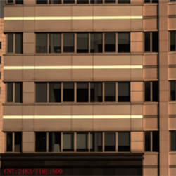
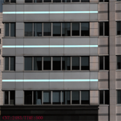
Figure 7. Color tranformation in lab and outdoor environment: (left) input image; (right) result.
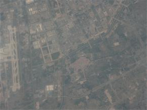


Figure 8. Radiometric calibration for Bayer video sequence (image is zoomed in for better analysis, covering Houston): (left) initial calibration (Bayer to RGB); (right) after no-uniformity correction from [7].
wind, the video is distorted and unstable. Therefore the video frames have to be stabilized for immediate object detection and real time surveillance. Video stabilization is a process to reduce the unwanted motion of the camera so as to remove the jitter and instability in the video frames [9].
Mechanical stabilization employs mechanical devices like gimbal to reduce the vibration of the structure holding the camera. However, this method is not able to reduce all the vibrations and is costly to implement. The Digital stabilization technique, however employs image processing based methods and can be used to remove the needless vibration that cannot be removed by Mechanical stabilization method. It costs less than the Mechanical technique as it does not involve complex hardware and requires only software to stabilize the video. Therefore digital stabilization is a better method of stabilization since it is inexpensive and easy to implement.
We noticed a parametric strategy in IPOL (www.ipol.im) with open source implementation [10], and used feature-based motion (homography) estimation with local matrix-based motion smoothing, and Figure 9 shows the basic framework.
For further approximately still video, we choose a registration method based on feature point to generate such product. SIFT [11] or ASIFT [12] feature descriptor can be used directly after receiving the stabilized sequences. Figure 10 shows the processed result for Marseille.
3.4. Video Compression
Although the compression standard is common in close range community, we got response from end user the compression always damage the expert analysis for small object, especially the high profile H.264 standard (it will incur small blocks near the edge and is of various compression ratios).
Hence, we limited the compression ration no more than 10 for interested region (or quality test video) and no more than 30 in other regions.

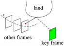
Figure 9. Illustration of the motion smoothing and imge registration. is the initial image, are the computed transformations. is the stabilized sequence and the stabilizing transformations [10].


Figure 10. Video stabilization and registration. Top: 20th frame; Bottom: 29th frame, some matching points. Notice the black border after global registration referred to given key frame (usually at nadir view point).
Table 2. SNR value using different object.
3.5. Geometric Processing
After building RPC file using attitude and GPS data, we can construct the L2 product mapped into a cartographic projection and corrected from sensor and terrain distortions. The mean value of geometrical location error is 500m after system correction and calibration (small satellite without high level star sensor).
Mosaic products will be automatically processed in order to provide end user with an ortho-image of larger size, this is vital for multi footprint mode.
4. Image Quality Evaluation
4.1. Module Transfer Function Value and SNR
We do not pave the traditional knife edge pattern (high cost) but find some natural object such as road or building to test the MTF value, showing in Figure 11.
Table 2 simply outlines the SNR result testified in different condition. Obvious difference can be seen the SNR value is not high while 45 db is common for TDI (Time delay integration) sensor, and explanation is the frame exposure time will not be long to balance DN value and fast moving object detection.
4.2. Video Stabilization Level
To quantify our video stabilization method, we carefully detect the matched feature points and calculate the residual error of every frame. In Figure12, it can be seen the average of error distance is reduced from largest 5 pixels to no more than 1 pixel in every frame after our processing, which prove its effectiveness (please go to Table 3).


Figure 11. MTF curve of OVS-1A (above) and OVS-1B (bottom). Bayer video mode lowers the MTF value from classical 0.1@Nyquist frequence to 0.08 and the blue channel decreas too fast.
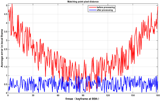
Figure 12. Average distance of matching points.
Table 3. Video stabilization error of different methods.
One thing should be kept in mind, this approach will not be used in video sequences with rare feature point, such as small ocean island, desert region.
5. Conclusions
OVS system is designed hoping to optimize the end user’s need. Its main image quality performances are ensured by appropriate processing line in end user’s production center (we worked on it for months).
Despite the success or progress, we noticed:
1) There are potential drawbacks to using color filter array (CFA) sensor such as Bayer filter, since CFA inherently lowers the resolution of the underlying staring sensor relative to a single spectrum image [2]. We are now designing more practical and effective system for overhead video system;
2) Video mode remote sensing lacks universal framework to guide how to construct the product, and end user usually cannot get the longitude or latitude from video product from any video player. We anticipate a full analysis to get an engineering product definition in the coming soon future.
After OVS-1A and OVS-1B, we successfully designed the TDI mode for area detector and extend the data picturing mode to traditional long strip.
Last but not least, Orbita has launched its newest video satellite with 0.9m resolution in 2018 July, and it can also be seen as another symbol for developing consumer remote sensing.
Acknowledgements
Thanks should be given to Senior Engineer Pan in Orbita for opening the data center to us.
This research has been partly supported by National Natural Science Foundation of China under Grant 61701023.
Conflicts of Interest
The authors declare no conflicts of interest regarding the publication of this paper.
Cite this paper
Cao, S.X., Qi, W.W., Tan, W., Zhou, N. and Hu, Y.F. (2018) Main Processes for OVS-1A & OVS- 1B: From Manufacturer to User. Journal of Computer and Communications, 6, 126-137. https://doi.org/10.4236/jcc.2018.611012
References
- 1. N2YO.com (October) ZHUHAI-1 02 (CAS 4B), Track ZHUHAI-1 02 (CAS 4B) Now! http://www.n2yo.com/satellite/?s=42759
- 2. Mann, J.M., Berkenstock, D. and Robinson, M.D. (2013) Systems and Methods for Overhead Imaging and Video. US Patent: No. 8487996B2.
- 3. Schowengerdt, R.A. (2013) Remote Sensing: Models and Methods for Image Processing. 3rd Edition, Academic Press, London.
- 4. Yin, S.M., Hong, X.H., Liu, S.Q. and Fu, X.N. (2004) New Algorithm of Adaptive Nonuniformity Correction for IRFPA. Journal of Infrared and Millimeter Waves, 23, 33-37. https://doi.org/10.3321/j.issn:1001-9014.2004.01.007
- 5. Zhao, X.Y., Zhang, W. and Xie, X.F. (2010) Study of Relationship between Absolute Calibration and Relative Calibration. Infrared, 31, 23-30. https://doi.org/10.3969/j.issn.1672-8785.2010.09.006
- 6. Friedenberg, A. and Goldblatt, I. (1998) Nonuniformity Two-Point Linear Correction Errors in Infrared Focal Plane Arrays. Optical Engineering, 37, 1251-1253. https://doi.org/10.1117/1.601890
- 7. Cao, S.X., Li, Y., Jiang, C. and Jia, G.R. (2017) Statistical Non-Uniformity Correction for Paddlebroom Thermal Infrared Image. Second International Conference on Multimedia and Image Processing, Wuhan, 17-19 March 2017, 1-5.
- 8. Wolf, S. (2003) Color Correction Matrix for Digital Still and Video Imaging Systems. National Telecommunications and Information Administration.
- 9. Kejriwal, L. and Singh, I. (2016) A Hybrid filtering approach of Digital Video Stabilization for UAV Using Kalman and Low Pass Filter. International Conference on Advances in Computing & Communications, 93, 359-366.
- 10. Sanchez, J. (2017) Comparison of Motion Smoothing Strategies for Video Stabilization Using Parametric Models. Image Processing Online, 1, 309-346. https://doi.org/10.5201/ipol.2017.209
- 11. Low, D. (2004) Distinctive Image Features from Scale-Invariant Keypoints. International Journal of Computer Vision, 60, 99-110. https://doi.org/10.1023/B:VISI.0000029664.99615.94
- 12. Morel, J.-M. and Yu G.S. (2009) ASIFT: A New Framework for Fully Affine Invariant Image Comparison. SIAM Journal on Imaging Sciences, 2, 438-469. https://doi.org/10.1137/080732730