Paper Menu >>
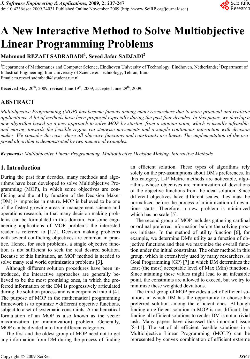
Journal Menu >>
 J. Software Engineering & Applications, 2009, 2: 237-247 doi:10.4236/jsea.2009.24031 Published Online November 2009 (http://www.SciRP.org/journal/jsea) Copyright © 2009 SciRes JSEA 237 A New Interactive Method to Solve Multiobjective Linear Programming Problems Mahmood REZAEI SADRABADI1, Seyed Jafar SADJADI2 1Department of Mathematics and Computer Science, Eindhoven University of Technology, Eindhoven, Netherlands; 2Department of Industrial Engineering, Iran University of Science & Technology, Tehran, Iran. Email: m.rezaei.sadrabadi@student.tue.nl Received May 20th, 2009; revised June 19th, 2009; accepted June 29th, 2009. ABSTRACT Multiobjective Programming (MOP) has become famous among many researchers due to more practical and realistic applications. A lot of methods have been proposed especially during the past four decades. In this paper, we develop a new algorithm based on a new approach to solve MOP by starting from a utopian point, which is usually infeasible, and moving towards the feasible region via stepwise movements and a simple continuous interaction with decision maker. We consider the case where all objective functions and constraints are linear. The implementation of the pro- posed algorithm is demonstrated by two numerical examples. Keywords: Multiobjective Linear Programming, Multiobjective Decision Making, Interactive Methods 1. Introduction During the past four decades, many methods and algo- rithms have been developed to solve Multiobjective Pro- gramming (MOP), in which some objectives are con- flicting and the utility function of the Decision Maker (DM) is imprecise in nature. MOP is believed to be one of the fastest growing areas in management science and operations research, in that many decision making prob- lems can be formulated in this domain. For some engi- neering applications of MOP problems the interested reader is referred to [1,2]. Decision making problems with several conflicting objectives are common in prac- tice. Hence, for such problems, a single objective func- tion is not sufficient to seek the real desired solution. Because of this limitation, an MOP method is needed to solve many real world optimization problems [3]. Although different solution procedures have been in- troduced, the interactive approaches are generally be- lieved to be the most promising ones, in which the pre- ferred information of the DM is progressively articulated during the solution process and is incorporated into it [4]. The purpose of MOP in the mathematical programming framework is to optimize r different objective functions, subject to a set of systematic constraints. A mathematical formulation of an MOP is also known as the vector maximization (or minimization) problem. Generally, MOP can be divided into four different categories. The first and the oldest group of MOP need not to get any information from DM during the process of finding an efficient solution. These types of algorithms rely solely on the pre-assumptions about DM's preferences. In this category, L-P Metric methods are noticeable, algo- rithms whose objectives are minimization of deviations of the objective functions from the ideal solution. Since different objectives have different scales, they must be normalized before the process of minimization of devia- tions starts. Therefore, a new problem is minimized which has no scale [5]. The second group of MOP includes gathering cardinal or ordinal preferred information before the solving proc- ess initiates. In the method of utility function [6], for example, we determine DM's utility as a function of ob- jective functions and then we maximize the overall func- tion under the initial constraints. The other method in this group, which is extensively used by many researchers, is Goal Programming (GP) [7] in which DM determines the least (the most) acceptable level of Max (Min) functions. Since attaining these values might lead to an infeasible point, the constraints are allowed to exceed, but we try to minimize these weighted deviations. The third group of MOP provides a set of efficient so- lutions in which DM has the opportunity to choose his preferred solution among the efficient ones. Although finding an efficient solution in MOP is not difficult, but finding all efficient solutions to render DM is not a trivial task. Many papers have discussed this important issue [8–11]. The set of all efficient feasible solutions in a Multiobjective Linear Programming (MOLP) can be represented by convex combination of efficient extreme 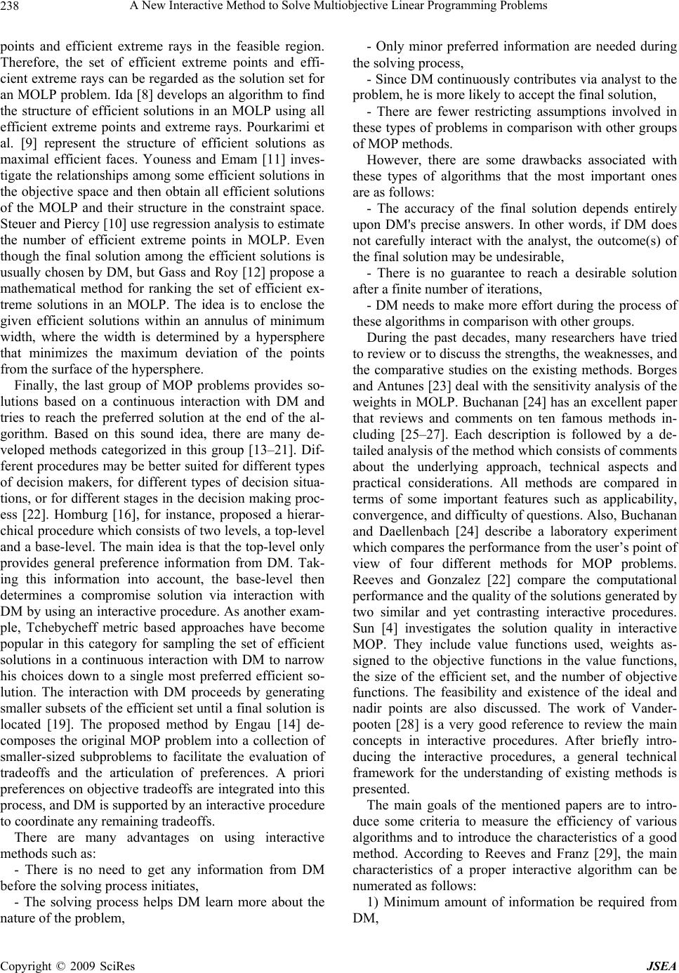 A New Interactive Method to Solve Multiobjective Linear Programming Problems 238 points and efficient extreme rays in the feasible region. Therefore, the set of efficient extreme points and effi- cient extreme rays can be regarded as the solution set for an MOLP problem. Ida [8] develops an algorithm to find the structure of efficient solutions in an MOLP using all efficient extreme points and extreme rays. Pourkarimi et al. [9] represent the structure of efficient solutions as maximal efficient faces. Youness and Emam [11] inves- tigate the relationships among some efficient solutions in the objective space and then obtain all efficient solutions of the MOLP and their structure in the constraint space. Steuer and Piercy [10] use regression analysis to estimate the number of efficient extreme points in MOLP. Even though the final solution among the efficient solutions is usually chosen by DM, but Gass and Roy [12] propose a mathematical method for ranking the set of efficient ex- treme solutions in an MOLP. The idea is to enclose the given efficient solutions within an annulus of minimum width, where the width is determined by a hypersphere that minimizes the maximum deviation of the points from the surface of the hypersphere. Finally, the last group of MOP problems provides so- lutions based on a continuous interaction with DM and tries to reach the preferred solution at the end of the al- gorithm. Based on this sound idea, there are many de- veloped methods categorized in this group [13–21]. Dif- ferent procedures may be better suited for different types of decision makers, for different types of decision situa- tions, or for different stages in the decision making proc- ess [22]. Homburg [16], for instance, proposed a hierar- chical procedure which consists of two levels, a top-level and a base-level. The main idea is that the top-level only provides general preference information from DM. Tak- ing this information into account, the base-level then determines a compromise solution via interaction with DM by using an interactive procedure. As another exam- ple, Tchebycheff metric based approaches have become popular in this category for sampling the set of efficient solutions in a continuous interaction with DM to narrow his choices down to a single most preferred efficient so- lution. The interaction with DM proceeds by generating smaller subsets of the efficient set until a final solution is located [19]. The proposed method by Engau [14] de- composes the original MOP problem into a collection of smaller-sized subproblems to facilitate the evaluation of tradeoffs and the articulation of preferences. A priori preferences on objective tradeoffs are integrated into this process, and DM is supported by an interactive procedure to coordinate any remaining tradeoffs. There are many advantages on using interactive methods such as: - There is no need to get any information from DM before the solving process initiates, - The solving process helps DM learn more about the nature of the problem, - Only minor preferred information are needed during the solving process, - Since DM continuously contributes via analyst to the problem, he is more likely to accept the final solution, - There are fewer restricting assumptions involved in these types of problems in comparison with other groups of MOP methods. However, there are some drawbacks associated with these types of algorithms that the most important ones are as follows: - The accuracy of the final solution depends entirely upon DM's precise answers. In other words, if DM does not carefully interact with the analyst, the outcome(s) of the final solution may be undesirable, - There is no guarantee to reach a desirable solution after a finite number of iterations, - DM needs to make more effort during the process of these algorithms in comparison with other groups. During the past decades, many researchers have tried to review or to discuss the strengths, the weaknesses, and the comparative studies on the existing methods. Borges and Antunes [23] deal with the sensitivity analysis of the weights in MOLP. Buchanan [24] has an excellent paper that reviews and comments on ten famous methods in- cluding [25–27]. Each description is followed by a de- tailed analysis of the method which consists of comments about the underlying approach, technical aspects and practical considerations. All methods are compared in terms of some important features such as applicability, convergence, and difficulty of questions. Also, Buchanan and Daellenbach [24] describe a laboratory experiment which compares the performance from the user’s point of view of four different methods for MOP problems. Reeves and Gonzalez [22] compare the computational performance and the quality of the solutions generated by two similar and yet contrasting interactive procedures. Sun [4] investigates the solution quality in interactive MOP. They include value functions used, weights as- signed to the objective functions in the value functions, the size of the efficient set, and the number of objective functions. The feasibility and existence of the ideal and nadir points are also discussed. The work of Vander- pooten [28] is a very good reference to review the main concepts in interactive procedures. After briefly intro- ducing the interactive procedures, a general technical framework for the understanding of existing methods is presented. The main goals of the mentioned papers are to intro- duce some criteria to measure the efficiency of various algorithms and to introduce the characteristics of a good method. According to Reeves and Franz [29], the main characteristics of a proper interactive algorithm can be numerated as follows: 1) Minimum amount of information be required from DM, Copyright © 2009 SciRes JSEA  A New Interactive Method to Solve Multiobjective Linear Programming Problems 239 2) The nature of decision making be simple, 3) If DM provides his answers improperly in some in- teractions, he can have the opportunity to compensate it in the following interactions, 4) The number of iterations to reach the final solution be reasonable, 5) DM be familiar with the nature of judgments he is asked for, 6) The algorithm be suitable for solving large scale problems. In this paper, we propose a new algorithm which is mainly in the group of interactive methods. However, we also need to get some information from DM before problem solving initiates; therefore, this algorithm is neither a pure interactive method nor a pure method in the second category. In addition, the proposed algorithm is based upon a novel approach to the problem, starting from an infeasible utopian point and moving towards the feasible region and then the final efficient point. The remaining of this paper is organized as follows. Section 2 provides some of the necessary definitions we need to use in this paper. In section 3, the problem statement and the proposed algorithm are explained. Two numerical examples are demonstrated in section 4 to illustrate the proposed algorithm. Finally, conclusion remarks appear in section 5 to summarize the contribution of the paper. 2. Definitions Consider an MOLP problem defined as follows, },...,2,1;0;|{ .. },...,2,1;)(max{ miXbXARXM ts rkXCXfZ ii n T kk (1) where, )(Xfk: is the kth objective function, k C: is the vector of coefficients in the kth objective function, X: is an n-dimensional vector of decision variables, i A: is the ith row of technological coefficients, i b: is the RHS of the ith constraint, and M: is the feasible region. A solution M X is efficient if and only if there does not exist another M X such that )()(XfXf kk for all and rk ,...,2,1)()(XfkXfk for at least one k. Then, the vector, },...,2,1);({ rkXfZ k (2) is called a non-dominated criterion vector. All efficient solutions in M form the efficient set E. Although some interactive algorithms search the entire feasible region M, the majority of them are designed to search only the effi- cient set E. The vector, },...,2,1);(max)(|)({ *** rkXfXfXfZ kkk (3) is called the ideal point or the ideal criterion vector. It should be mentioned that the ideal criterion vector, and so the ideal solution , does not usually exist. The vector, * X },...,2,1);(max)(|)({ ****** rkXfXfXfZ kkk (4) is called a utopian vector or a utopian point. Unlike the ideal criterion vector, there exist many utopian vectors. Nevertheless, their corresponding ** X ’s are most likely infeasible. 3. Problem Statement The majority of methods proposed in the domain of in- teractive procedures search the feasible region M or the efficient set E through interaction with DM in order to attain the final solution. Here, we develop a new algo- rithm to solve MOLP problems by starting from a uto- pian point ** X (which is usually infeasible) and mov- ing towards the feasible region M and then the efficient set E via stepwise movements and a plain continuous interaction with DM in order to be in line with his pref- erences. Since there are many utopian points outside the M, we choose the clst ** ose X to M as the start point, by considering the least sum of weighted deviations from the constraints. 3.1 The Proposed Algorithm The proposed algorithm attains an efficient solution of an MOLP through the following steps: Algorithm: Step 1. Ask DM to determine, the maximum ac- ceptable reduction in the amount of in any interac- tion. Also, ask him to determine, a penalty for devia- tion of each unit from the ith constraint. In the next step, we find a utopian point allowing some deviations from the constraints , in that the utopian point maybe a point with some negative’s. However, we also con- sider a big penalty, k a i w k f 0 j x w j x , for each unit of such deviations. Step 2. Maximize each with consideration of the feasible set M as follows, )(Xfk },...,2,1;0;|{ .. )(max miXbXARXM ts XCXf ii n T kk (5) Step 3. Let be the optimal solution for )(* Xfk Copyright © 2009 SciRes JSEA  A New Interactive Method to Solve Multiobjective Linear Programming Problems 240 each . Solve the following GP prob- lem, rkXfk,...,2,1);( 1;,...,2,1 ; min{ 1 jmi xdbXA wdw jiii m i ii i d },...,2,1;,...,2, ;0; );()(|* 1 rkn dd XfXfd j kk n j j (6) where, represents the deviation from the ith con- straint. In this step, we allow our solution to go outside the feasible region. Suppose X is the solution for (6). Set X X ik 0 and go to step 4. Step 4. Let be the angle between and . Calculate i fk f ik sin as follows, ||.|| . 1 ki ki CC CC sinik (7) Now, we can determine a small step δ by which we move towards the feasible region in each iteration as, };,...,2,1,; sin|| min{ kirki C a iki i (8) Step 5. Consider constraints which remain active. Now ask DM to see which active objec- tive has the least desirability. Let l be the index for the which has the least desirability. )()( *0 XfXf kk l f Step 6. Solve the following optimization problem in which we take a step δ from 0 X towards the feasible region while we keep the amount of , l f },...,2,1;,...,2,1 ;0;;||; );()(|min{ 0 0 11 njmi ddxXXdbXA XfXfdwdw jjiii ll n j j m i ii (9) where, |.| is the 2-norm. In this step there is no change in the value of but we usually expect that the other objective functions get worse, but not necessarily. In other words, we might encounter a situation in which the values of some active or inactive get better. l f k f Step 7. If then go to step 8, otherwise set 0 11 n j j m i ii dwdw X X 0, calculate the new values of , and go to step 5. )( 0 Xfk Step 8. implies that we are in- side the feasible region, but most likely not on the boundary. Therefore, we take a smaller step to be stopped on the boundary by solving, 0 11 n j j m i ii dwdw },...,2,1;,...,2,1;,...,2,1 ;0;);()(| |min{|00 rknjmi xbXAXfXfXX jiikk (10) There is no guarantee that the solution of step 8 is a non-dominated one. So, we move on the boundary to reach a non-dominated solution. Set X X 0, },...,2,1{ rS , and go to step 9. Step 9. Ask DM to see which objective in S has the least desirability. Let l be the index for the which has the least desirability. Solve the following optimiza- tion problem in which we take a step at most with the amount of δ from l f 0 X on the boundary of the feasible region while we keep the amounts of , rkfk1; ,...,2, },...,2,1;,...,2,1;,...,2,1;0 ;||;);()(|)(max{ 00 rknjmix XXbXAXfXfXf j iikkl (11) Step 10. If then set )()( 0 XfXfll },...,2,1{ rS and go to step 9, otherwise set and go to step 11. lSS Step 11. If S then choose X as the final efficient solution, otherwise set X X 0 and go to step 9. End. It should be noted that steps 1-8 help us to reach to the feasible region M by starting from the closest utopian point in line with DM’s preferences, whereas steps 9-11 guarantee that the final solution is an efficient one, i.e., the final solution is in E. 3.2 Some Lemmas to Determine δ Here, we show how to choose δ in Step 4 of the proposed algorithm with the following three lemmas. Lemma 1: Any step δ along gradient vector will result a decrease (or increase) of k C || k C in . k f Proof: Let kj be the angle between and axis k C j x . Therefore, || 1|| )0,...,1,...,0).(,...,,...,( |||| . cos 1 k kj k knkjk jk jk kj C c C ccc xC xC (12) where, is the jth unique vector in an n-dime- nsional space. The angle between j x k C and j x helps us to compute the projection of k C over the axis j x , i.e., Copyright © 2009 SciRes JSEA  A New Interactive Method to Solve Multiobjective Linear Programming Problems 241 if we take a step δ along vector k C , the amount of change in each element of j x is kj cos or )cos( kj depending on the direction we choose. Figure 1 depicts the gradient vector k C and its projec- tion in a 2-dimensional space. Therefore, | k kj |C c cos kjj x (13) or || cos )cos( k kj kj C c kjj x k f (14) Therefore, we can compute the change in the amount of as follows, ||.| | ..|| 2 1 2 11 kk k n j kj k n j kj n j jkjk CC C c C cxcf |. || || k kj l |C c C (15) We now present a generalized form of Lemma (1). Lemma 2: Any step δ along which makes the angle lk with will result a decrease (increase) of k C lkk C cos|| in . k f Proof: It is clear that taking a step δ along which makes the angle l C lk with is the same as taking a k C Figure 1. The gradient vector k C and its projection (a) (b) Figure 2. Demonstration of taking a step δ on in a 2-dimensional space l H step lk cos along . Using the results of Lemma(1) yields, k C ||cos|| klkk Cf (16) Lemma 3: Let be a hyperplane which is or- thogonal to l and makes the angle l H l CC lk with . Any step δ on the hyperplane in any direction will result a decrease (increase) of k C l H sin|| klk C in . k f Proof: We prove this lemma in two steps. In the first step, let 2/0 lk , then taking any step δ on l H in any direction is the same as taking a step δ in the direction whose angle with is l C2/ and there- fore makes the angle lk 2/ with . Figure 2(a) demonstrates the situation in a 2-dimensional space. k C According to lemma (2), taking any step δ along the direction which makes the angle lk 2/ or lk 2/ with will result a change with the amount of k C 2/ ||)cos(klk C or ||)2/ lk cos( k C in . Since k f 2/0 lk , we have, ||sin||)2/cos( klkklk CC (17) or ||sin||)2/cos( klkklk CC (18) Finally, we have, ||sin|| klkk Cf (19) Now, in the second step, suppose lk 2/ k C . Taking any step δ on in any direction is the same as taking a step δ in the direction whose angle with is l H 2/ lk or lk 2/3 . Figure 2(b) demonstrates the situation in a 2-dimensional space. Using similar argu- ment used in the first step yields, ||sin||)2/cos( klkklk CC (20) or ||sin||)2/3cos(klkklk CC (21) Finally, we have, ||sin|| klkk Cf (22) Now, we are ready to determine the amount of δ prop- erly. Suppose DM determines that he wouldn't expect any reduction more than in the amount of in any interaction. When we perform step (4) in the algo- rithm, actually we keep unchanged. In order to k a l f k f Copyright © 2009 SciRes JSEA  A New Interactive Method to Solve Multiobjective Linear Programming Problems 242 achieve this goal, we have to take step δ on . Ac- cording to lemma (3), the step leads to an increase (de- crease) l H ||sin klkC in . There is no problem in our approach in case increases. However, we must ensure that the step δ would not worsen more than , which suggest to keep the following condition, k f kak k f k f l k a krCklk | ;,...,1;|sin (23) or lkr;,...,1k lk ; C a k k || l f sin k a k (24) Holding (19) in all interactions throughout the algo- rithm guarantees that there would be no reduction in any more than . Since DM is entitled to keep the amount of any , the following condition must hold in order to obtain an appropriate δ, kfk; lk rl ;,...,1,k lk ; C a k || k sin (25) Finally, we are about to determine the best amount of δ with consideration of DM’s intentions and concurrently reaching to the feasible solution by doing as fewer inter- actions as possible. Thus, we have, }l;kr,...,1,; lk sin lk k 0 5 15 4 5 2 2 2 1 x x x x x | a k .6 9 2 1 2 1 x | min{ C , 22 7 .. 1 1 1 1 x x x x x ts Maxz Maxz (26) 4. Numerical Examples In this section we demonstrate implementation of the proposed method using two numerical examples. 4.1 Example 1 Consider the following MOLP problem with two objec- tive functions, 165 63 20 2 6 21 2 x x (27) We first ask DM to specify his sensitivity about the constraints and the objectives. As we already defined, ’s are the penalties associated with the constraints and ’s are the permitted amounts of reduction on the ob- jective functions in each iteration. For the sake of sim- plicity suppose that all constraints have equal sensitivity, i.e., i w k a 4,...,1;1 iwi. Next, we have to determine the acceptable amount of reduction on the objectives 1 z and 2 z . For this example, suppose DM specifies 2 and 3 for and , respectively. The appropriate value for δ can be determined as the following, 1 a2 a 3761||) 22 1 C6,1( 1C 2925||) 22 2 C2,5( 2C 52.0 29.37 )2,5).(6,1( ||.|| cos 12 C . 21 21 C CC 85.0)52.0(1sin12 2 38.0} )85.0(29 3 , )85.0( 2 } sin|| , sin| 212 2 121 1 C aa 37 min{ | min{ C Then, we must find and . Solving two distinct LP problems with consideration of and yields * 1 z* 2 z 1 z2 z ) 49.1(,(1.5,95) 2 xx with 86.34 * 1 z and)47.1,50), 2.6(( 1 xx with , respectively. In the next step, we ob- tain the utopian point in which both objectives are satis- fied at least with their optimal values, while we reach to a common point. Hence, we have, 43. ;0 : 2 6 5.6 9 4 2 2 1 i x d d x x x ) ** 2 35 * 2 z (* 1 6,...,1 , 43.355 86.34 1651522 637 20 .. )(1000 1 62 51 21 1 41 32 221 121 654321 d signinfreex x x x x dx dxx dx dxx ts ddddddMinD i (28) The optimal solution for (28) is with )96.4,10.5(),( ** 2 ** 1xx )43.35,86.34(, * z 2 z z and . In the next step, the DM is asked to select the objective which has the least desirability for him. Suppose in the first interaction the DM adopts . Therefore, we must solve the following problem, 02.39 ** D Copyright © 2009 SciRes JSEA  A New Interactive Method to Solve Multiobjective Linear Programming Problems 243 6,...,1;0 :, 38.0)96.4()10.5( 43.3525 5.6 1651522 6397 204 .. )(1000 21 2 2 2 1 21 62 51 41 321 221 121 654321 id signinfreexx xx xx dx dx dx dxx dxx dxx ts ddddddMinD i (29) The optimal solution for (29) is with and . Table 1 summarizes the results of implementation of the pro- posed algorithm during the next iterations. )61.4,24.5(),( 21 xx 65.34D)43.35,89.32(),(22 zz As one can observe, we have reached to the feasible region after 8 iterations. The final step by which we reach to the feasible region is from 12 ,xx (4.04, 4.10) to with feasible amounts . So, in order to reach to the fea- sible region by a smaller step we solve, )75.3,18.4(),( 21xx )38.28,65.26(),( 21 zz Table 1. The detailed information for implementation of the proposed method for example 1 Iteration Objective x1 x2 D z1 z2 0 max z1 1.95 5.49 0 34.8620.73 0 max z2 6.5 1.47 0 15.3235.43 0 utopian 5.1 4.96 39.02 34.8635.43 1 keep z2 5.24 4.61 34.65 32.8935.43 2 keep z2 5.38 4.25 30.27 30.8835.43 3 keep z1 5.01 4.32 20.9 30.8833.69 4 keep z2 5.17 3.91 15.87 28.6333.69 5 keep z1 4.8 3.97 6.5 28.6331.94 6 keep z1 4.42 4.04 4.28 28.6330.18 7 keep z1 4.04 4.1 2.14 28.6328.38 8 keep z2 4.18 3.75 0 26.6528.38 9 min delta 4.17 3.75 0 26.6928.38 10 max z1 4.17 3.75 0 26.6928.38 11 max z2 4.17 3.75 0 26.6928.38 2,1;0 5.6 1651522 6397 204 38.2825 65.266 .. )10.4()04.4( 1 21 21 21 21 21 2 2 2 1 jx x xx xx xx xx xx ts xxMinD j (30) Problem (30) leads to, with )75.3,17.4(),(21 xx )38.28,69.26(),( 21 zz and 37.0 , which is the first feasible point on the boundary of the feasible region. Then, the DM is asked to determine the objective func- tion which has the least desirability. Suppose he adopts , so we solve, 1 z 2,1;0 5.6 1651522 6397 204 38.2825 38.0)75.3()17.4( .. 6 1 21 21 21 21 2 2 2 1 211 jx x xx xx xx xx xx ts xxMaxz j (31) Problem (31) leads to with )75.3,17.4(),(21 xx )38.28,69.26(),( 21 zz }2{ . As one can see, cannot be improved by moving from . So, we have 1 z )75.3,17.4(), 21 xx( S2 z and is chosen to get improved. We solve, 2,1;0 5.6 1651522 6397 204 69.266 38.0)75.3()17.4( .. 25 1 21 21 21 21 2 2 2 1 212 jx x xx xx xx xx xx ts xxMaxz j (32) Problem (32) leads to with )75.3,17.4(),(21 xx )38.28,69.26(),( 21 zz . As one can see, cannot be improved by moving from . So, 2 z )75.3,17.4(),(21 xx Copyright © 2009 SciRes JSEA  A New Interactive Method to Solve Multiobjective Linear Programming Problems Copyright © 2009 SciRes JSEA 244 S 21,zz and with is the final efficient feasible solution. )75.3,17.4(),( 21 xx 0,..., 2516 103 401320 2572 576 .. 58 76 8010 41 321 321 321 321 321 213 212 11 xx xxx xxx xxx xxx xxx ts xxMaxz xxMaxz xMaxz 321 ,,, www 1000 w 3 z )38.28,69.26(),(21 zz 228 15 800 320 142 4 8 1625 4 43 43 43 x xx xx xx 5 w 4.2 Example 2 Consider the following MOLP problem with three objec- tive functions, 80 24 16 9 3 12 25 4 4 4 4 2 x x x x x (33) Suppose that the values 12, 5, 45, 2, and 6 are speci- fied by the DM for , and , respectively and we consider . Also, 300, 50, and 30 are determined as the acceptable amount of reduction for , and . The optimal value for δ is determined as follows, 4 w 7350||)15,25,80,10( 11 CC 774||)8,25,7,6(22 C C 249||)4,12,5,8( 23 C C 82.0)57.0(1sin 57.0 774.7350 )8,25,7,6).(15,25,80,10( ||.|| . 2 12 21 21 12 CC CC cos 1)03.0(1sin 03.0 249.7350 )4,12,5,8).(15,25,80,10( ||.|| . 2 13 31 31 13 CC CC cos 62.0)79.0(1sin 79.0 249.774 )4,12,5,8).(8,25,7,6( ||.|| . 2 23 32 32 23 CC CC cos 90.1 ,90.1,90.2,19.2,50.3,27.4min{} sin|| , , sin|| , sin|| , sin|| , sin|| min{ 323 3 31 232 2 212 2 131 1 121 1 C a C a C a C a C a }07.3 sin|| 3 3 C a Now, , and must be found. Solving three LP problems with consideration of , and sepa- rately yields * 2 * 1,zz * 3 z , 2 21,zz .35,22. 3 z )0,0,0517(),,( 431 xx 20.10,.16(),,( 41 xx ,32 with , 87.2975 * 1z)0,52.4,66 xxx 3,0,0),,( 43xx x ,21xx with , and with , respectively. Then, we obtain the utopian point in which three objectives are satisfied at least with their optimal values while we reach to a common point. Therefore, we have, 64.386 * 2z)98.,82.36( 45.310 * 3z ;0 :,..., 58 76 8010 516 103 1320 72 76 .. (1000 41 94 83 72 61 21 21 1 1 1 1 21 1 6 id xx dx dx dx dx xx xx x xx xx x xx x ts d MinD i ,( ** 1 9,...,1 45.310412 64.386825 87.29751625 228802 1524 8001640 320925 14235 ) 6245512 43 43 432 5432 4432 3432 243 1432 987 54321 signinfree xx xx xxx dxx dxx dxxx dx x dxxx ddd ddddd (34) The optimal solution is with )0,0,30,56.57(),,,( ** 4 ** 3 ** 2 ** 1xxxx )48.310,36.555,60.2975(), ** 3 ** 2 z 43 and zz .33380 ** D 1 z3 z . In the next step, the DM is asked to select the objective which has the least desirability for him. Since the constraint associated with 2 is not ac- tive, the DM is allowed to select one of the objectives or to keep its value. Suppose in the first iteration the DM adopts . Therefore, the following problem should be solved, z 3 z 9,...,1;0 :,..., 9.1 )0()0()30()56.57( 48.31041258 228802516 1524103 80016401320 32092572 1423576 .. )(1000 6245512 41 2 4 2 3 2 2 2 1 4321 94 83 72 61 54321 44321 34321 24321 14321 9876 54321 id signinfreexx xxxx xxxx dx dx dx dx dxxxx dxxxx dxxxx dxxxx dxxxx ts dddd dddddMinD i (35)  A New Interactive Method to Solve Multiobjective Linear Programming Problems 245 Table 2. The detailed information for implementation of the proposed method for example 2 Iteration Objective x1 x2 x3 x4 D z1 z2 z3 0 max z1 17.22 35.05 0 0 0 2976.2 348.67 -37.49 0 max z2 16.66 4.52 10.2 0 0 783.2 386.6 233.08 0 max z3 36.82 0 0 3.98 0 431.88 252.76 310.48 0 utopian 57.56 30 0 0 33380.43 2975.6 555.36 310.48 1 keep z3 56.74 28.29 -0.17 0 31484.82 2826.35 534.22 310.48 2 keep z3 55.92 26.58 -0.33 0 29613.44 2677.35 513.33 310.48 3 keep z1 54.4 27.09 -1.35 0 27726.82 2677.35 482.28 283.55 4 keep z3 53.58 25.38 -1.52 0 25860.25 2528.2 461.14 283.55 5 keep z3 52.76 23.67 -1.68 0 23988.88 2379.2 440.25 283.55 6 keep z3 51.94 21.96 -1.85 0 22118.36 2229.95 419.11 283.55 7 keep z3 51.12 20.25 -2.02 0 20244.01 2080.7 397.97 283.55 8 keep z1 49.6 20.76 -3.04 0 18351.77 2080.7 366.92 256.52 9 keep z1 48.08 21.27 -4.06 0 16465.06 2080.7 335.87 229.57 10 keep z3 47.26 19.56 -4.23 0 14599.55 1931.65 314.73 229.57 11 keep z3 46.44 17.85 -4.39 0 12728.18 1782.65 293.84 229.57 12 keep z3 45.62 16.14 -4.56 0 10857.66 1633.4 272.7 229.57 13 keep z1 44.1 16.65 -5.58 0 8965.42 1633.4 241.65 202.59 14 keep z1 42.58 17.16 -6.6 0 7078.71 1633.4 210.6 175.64 15 keep z3 41.12 16.21 -5.83 0 5830.92 1562.25 214.44 177.95 16 keep z3 39.75 15.32 -4.86 0 4855.56 1501.6 224.24 183.08 17 keep z3 38.38 14.43 -3.88 0 3882.43 1441.2 234.29 188.33 18 keep z2 37.01 13.54 -2.91 0 2906.67 1380.55 244.09 193.46 19 keep z2 35.64 12.65 -1.93 0 1933.53 1320.15 254.14 198.71 20 keep z1 33.95 12.59 -1.07 0 1066.54 1320.15 265.08 195.81 21 keep z1 32.26 12.53 -0.2 0 203.27 1320.15 276.27 193.03 22 keep z1 30.45 12.59 0 0.52 0 1320.15 274.99 182.73 23 min delta 31.86 12.52 0 0 0 1320.2 278.8 192.28 24 max z1 31.86 12.52 0 0 0 1320.2 278.8 192.28 25 max z2 31.85 12.52 0 0 0 1320.2 278.8 192.28 26 max z3 31.86 12.52 0 0 0 1320.2 278.8 192.28 The optimal solution for (35) is with ),,,(4321 xxxx )0,17.0,29.28,74.56( )43.310,22.534,35.2826(),,(321 zzz and . 82.31484D Table 2 summarizes the results of implementation of the proposed algorithm for example 2. Note that the con- straint associated with is not active till iteration 8. Therefore, he is allowed to choose 2 z 2 z as the objective whose desirability is the least amount from iteration 8. According to Table 2, we reach to the feasible region in iteration 22. So, solving the following problem helps us to attain the boundary of the feasible region, 4,...,1;0 228802516 1524103 80016401320 32092572 1423576 73.18241258 99.27482576 02.132016258010 .. )0()2.0()53.12()26.32( 4321 4321 4321 4321 4321 4321 4321 4321 2 4 2 3 2 2 2 1 jx xxxx xxxx xxxx xxxx xxxx xxxx xxxx xxxx ts xxxxMinD j (36) Copyright © 2009 SciRes JSEA  A New Interactive Method to Solve Multiobjective Linear Programming Problems 246 The optimal solution for (36) is ),,,( 4321 xxxx )28.192,8.278,2. with and )0,0,52.12,86.31( 44.0 1320(),,( 321 zzz . Suppose the DM adopts as the objective to get improved. Hence, 1 z 4,...,1;0 228802516 1524103 80016401320 32092572 1423576 73.18241258 99.27482576 9.1)0()2.0()53.12()26.32( .. 16258010 4321 4321 4321 4321 4321 4321 4321 2 4 2 3 2 2 2 1 43211 jx xxxx xxxx xxxx xxxx xxxx xxxx xxxx xxxx ts xxxxMaxz j (39) The optimal solution for (39) is ),,,( 4321 xxxx )28.192,8.278, )with . Since 0,0,52.12,86.31( 1 2.1320(),,( 321 zzz z does not change, we have . Then, }3,2{S 2 z is adopted by the DM to get improved, which leads to, 4,...,1;0 228802516 1524103 80016401320 32092572 1423576 73.18241258 2.132016258010 9.1)0()2.0()53.12()26.32( .. 82576 4321 4321 4321 4321 4321 4321 4321 2 4 2 3 2 2 2 1 43212 jx xxxx xxxx xxxx xxxx xxxx xxxx xxxx xxxx ts xxxxMaxz j (40) The optimal solution for (40) is ),,,( 4321 xxxx )28.192,8.278,2. with . Obviously, )0,0,52.12,86.31( 2 1320(),,(321 zzz z remains unchanged; so, . The only remaining objective is and we have, }3{S 3 z 4,...,1;0 228802516 1524103 80016401320 32092572 1423576 8.27882576 2.132016258010 9.1)0()2.0()53.12()26.32( .. 41258 4321 4321 4321 4321 4321 4321 4321 2 4 2 3 2 2 2 1 43213 jx xxxx xxxx xxxx xxxx xxxx xxxx xxxx xxxx ts xxxxMaxz j (41) The optimal solution for (41) is ),,,( 4321 xxxx )28.192,8.278,2. 3 z ) with . Since similar to and , the amount of remains unchanged, we have 0,0,52.12,86.31(1320(),,( 321 zzz 2 z 1 z S (),,,( 4321 xxxx )28.192,8.278,2.1320 . Therefore, the final efficient feasible solution is with )0,0,52.12,86.31 (),,( 321 zzz . 5. Conclusions We have proposed a new interactive algorithm to solve MOLP in which we need some initial information about DM's preferences. Unlike the majority of interactive methods, the proposed method starts from the utopian point, which is usually infeasible, and moves towards the feasible region and the efficient set. Based on the results of some proved lemmas, we are able to specify the amount of steps towards the feasible region. Our method satisfies most of the characteristics that a good interac- tive method needs, such as simplicity of the nature of judgments for DM, having the opportunity to compensate improper decisions in previous interactions, and handling his nonlinear utility. Implementation of the proposed method has been demonstrated by using two numerical examples. REFERENCES [1] F. B. Abdelaziz, “Multiple objective programming and goal programming: New trends and applications,” Euro- pean Journal of Operational Research, Vol. 177, pp. 1520–1522, 2007. [2] M. M. Wiecek, “Multiple criteria decision making for engineering,” Omega, Vol. 36, pp. 337–339, 2008. [3] J. Kim and S. K. Kim, “A CHIM-based interactive Tche- bycheff procedure for multiple objective decision mak- ing,” Computers & Operations Research, Vol. 33, pp. 1557–1574, 2006. [4] M. Sun, “Some issues in measuring and reporting solu- tion quality of interactive multiple objective programming procedures,” European Journal of Operational Research, Vol. 162, pp. 468–483, 2005. [5] M. Zeleny, “Multiple criteria decision making,” MC Graw-Hill, New York, 1982. [6] R. Kenney and H. Raiffa, “Decisions with multiple objec- tives: Preferences and value trade-offs,” J. Wiley, New York, 1976. [7] C. Romero, “Handbook of critical issues in goal pro- gramming,” Pergamon Press, Oxford, 1991. [8] M. Ida, “Efficient solution generation for multiple objec- tive linear programming based on extreme ray generation method,” European Journal of Operational Research, Vol. 160, pp. 242–251, 2005. [9] L. Pourkarimi, M. A. Yaghoobi and M. Mashinchi, “De- termining maximal efficient faces in multiobjective linear programming problem,” Journal of Mathematical Analy- Copyright © 2009 SciRes JSEA  A New Interactive Method to Solve Multiobjective Linear Programming Problems Copyright © 2009 SciRes JSEA 247 sis and Applications, Vol. 354, pp. 234–248, 2009. [10] R. E. Steuer and C. A. Piercy, “A regression study of the number of efficient extreme points in multiple objective linear programming,” European Journal of Operational Research, Vol. 162, pp. 484–496, 2005. [11] E. A. Youness and T. Emam, “Characterization of effi- cient solutions for multi-objective optimization problems involving semi-strong and generalized semi-strong e-convexity,” Acta Mathematica Scientia, Vol. 28B(1), pp. 7–16, 2008. [12] S. I. Gass and P. G. Roy, “The compromise hypersphere for multiobjective linear programming,” European Jour- nal of Operational Research, Vol. 144, pp. 459–479, 2003. [13] J. Chen and S. Lin, “An interactive neural network-based approach for solving multiple criteria decision making problems,” Decision Support Systems, Vol. 36, pp. 137–146, 2003. [14] A. Engau, “Tradeoff-based decomposition and deci- sion-making in multiobjective programming,” European Journal of Operational Research, Vol. 199, pp. 883–891, 2009. [15] L. R. Gardiner and R. E. Steuer, “Unified interactive mul- tiple objective programming,” European Journal of Op- erational Research, Vol. 74, pp. 391–406, 1994. [16] C. Homburg, “Hierarchical multi-objective decision mak- ing,” European Journal of Operational Research, Vol. 105, pp. 155–161, 1998. [17] C. L. Hwang and A. S. M. Masud, “Multiple objective decision making methods and applications,” Springer- Verlag, Amsterdam, 1979. [18] B. Malakooti and J. E. Alwani, “Extremist vs. centrist decision behavior: Quasi-convex utility functions for in- teractive multi-objective linear programming problems,” Computers & Operations Research, Vol. 29, pp. 2003– 2021, 2002. [19] G. R. Reeves and K. R. MacLeod, “Some experiments in Tchebycheff-based approaches for interactive multiple objective decision making,” Computers & Operations Research, Vol. 26, pp. 1311–1321, 1999. [20] R. E. Steuer, J. Silverman, and A. W. Whisman, “A com- bined Tchebycheff/aspiration criterion vector interactive multi-objective programming procedure,” Computers & Operations Research, Vol. 43, pp. 641–648, 1995. [21] M. Sun, A. Stam, and R. E. Steuer, “Interactive multiple objective programming using Tchebycheff programs and artificial neural networks,” Computers & Operations Re- search, Vol. 27, pp. 601–620, 2000. [22] G. R. Reeves and J. J. Gonzalez, “A comparison of two interactive MCDM procedures,” European Journal of Operational Research, Vol. 41, pp. 203–209, 1989. [23] A. R. P. Borges and C. H. Antunes, “A visual interactive tolerance approach to sensitivity analysis in MOLP,” European Journal of Operational Research, Vol. 142, pp. 357–381, 2002. [24] J. T. Buchanan and H. G. Daellenbach, “A comparative evaluation of interactive solution methods for multiple objective decision models,” European Journal of Opera- tional Research, Vol. 29, pp. 353–359, 1987. [25] A. A. Geoffrion, J. S. Dyer, and A. Feinberg, “An inter- active approach for multi-criterion optimization with an application to the operation of an academic department,” Management Science, Vol. 19, pp. 357–368, 1972. [26] R. E. Steuer and E. U. Choo, “An interactive weighted Tchebycheff procedure for multiple objective program- ming,” Mathematical Programming, Vol. 26, pp. 326–344, 1983. [27] S. Zionts and J. Wallenius, “An interactive multiple ob- jective linear programming method for a class of under- lying nonlinear utility functions,” Management Science, Vol. 29, pp. 519–529, 1983. [28] D. Vanderpooten, “The interactive approach in MCDA: A technical framework and some basic conceptions,” Mathematical and Computer Modelling, Vol. 12, pp. 1213–1220, 1989. [29] G. R. Reeves and L. Franz, “A simplified interactive mul- tiple objective linear programming procedure,” Com- puters and Operations Research, Vol. 12, pp. 589–601, 1985. |