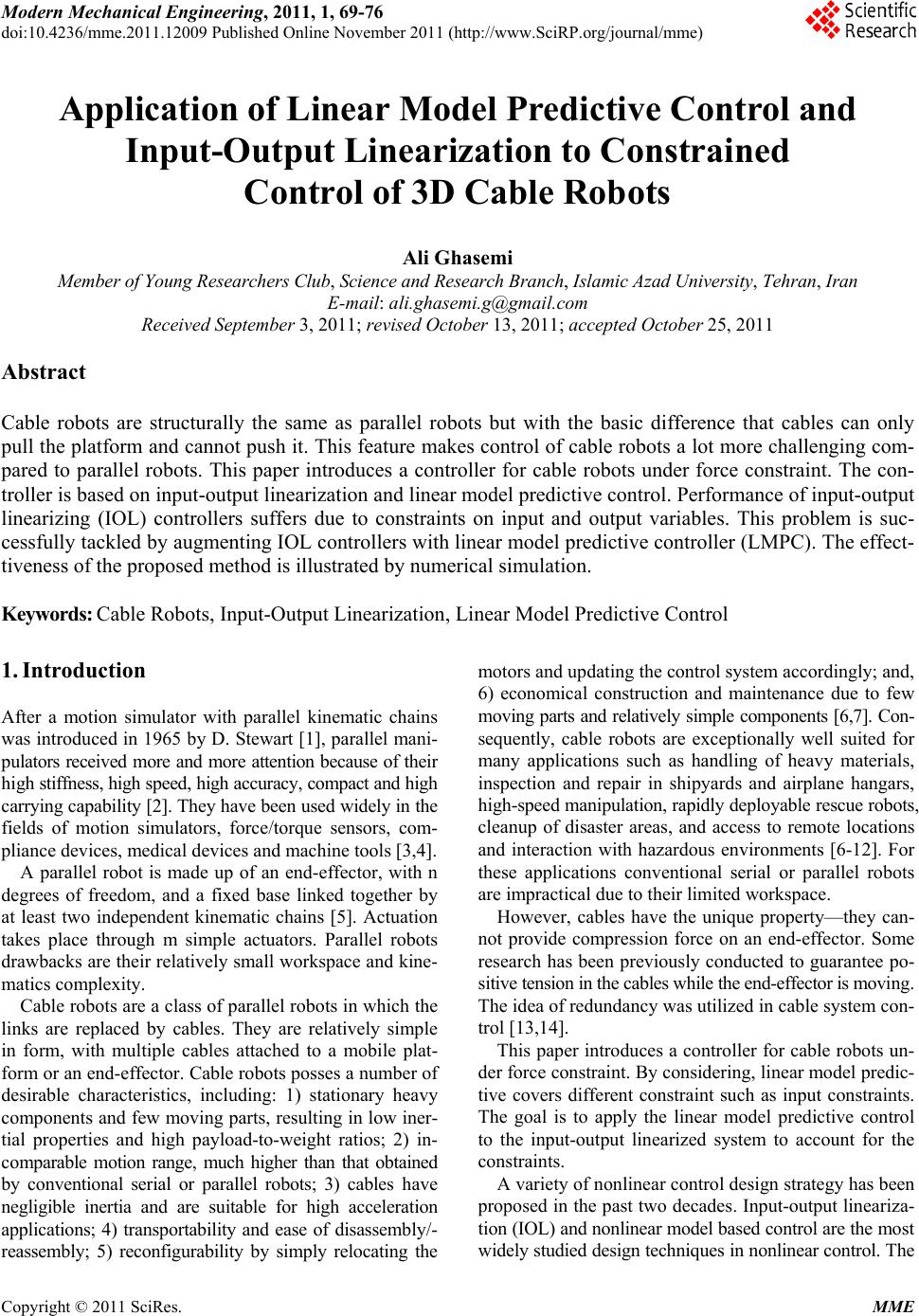Modern Mechanical Engineering, 2011, 1, 69-76
doi:10.4236/mme.2011.12009 Published Online November 2011 (http://www.SciRP.org/journal/mme)
Application of Linear Model Predictive Control and
Input-Output Linearization to Constrained
Control of 3D Cable Robots
Ali Ghasemi
Member of Young Researchers Club, Science and Research Branch, Islamic Azad University, Tehran, Iran
Received September 3, 2011; revised October 13, 2011; accepted October 25, 2011
Abstract
Cable robots are structurally the same as parallel robots but with the basic difference that cables can only
pull the platform and cannot push it. This feature makes control of cable robots a lot more challenging com-
pared to parallel robots. This paper introduces a controller for cable robots under force constraint. The con-
troller is based on input-output linearization and linear model predictive control. Performance of input-output
linearizing (IOL) controllers suffers due to constraints on input and output variables. This problem is suc-
cessfully tackled by augmenting IOL controllers with linear model predictive controller (LMPC). The effect-
tiveness of the proposed method is illustrated by numerical simulation.
Keywords: Cable Robots, Input-Output Linearization, Linear Model Predictive Control
1. Introduction
After a motion simulator with parallel kinematic chains
was introduced in 1965 by D. Stewart [1], parallel mani-
pulators received more and more attention because of their
high stiffness, high speed, high accuracy, compact and high
carrying capability [2]. They have been used widely in the
fields of motion simulators, force/torque sensors, com-
pliance devices, medical devices and machine tools [3,4].
A parallel robot is made up of an end-effector, with n
degrees of freedom, and a fixed base linked together by
at least two independent kinematic chains [5]. Actuation
takes place through m simple actuators. Parallel robots
drawbacks are their relatively small workspace and kine-
matics complexity.
Cable robots are a class of parallel robots in which the
links are replaced by cables. They are relatively simple
in form, with multiple cables attached to a mobile plat-
form or an end-effector. Cable robots posses a number of
desirable characteristics, including: 1) stationary heavy
components and few moving parts, resulting in low iner-
tial properties and high payload-to-weight ratios; 2) in-
comparable motion range, much higher than that obtained
by conventional serial or parallel robots; 3) cables have
negligible inertia and are suitable for high acceleration
applications; 4) transportability and ease of disassembly/-
reassembly; 5) reconfigurability by simply relocating the
motors and updating the control system accordingly; and,
6) economical construction and maintenance due to few
moving parts and relatively simple components [6,7]. Con-
sequently, cable robots are exceptionally well suited for
many applications such as handling of heavy materials,
inspection and repair in shipyards and airplane hangars,
high-speed manipulation, rapidly deployable rescue robots,
cleanup of disaster areas, and access to remote locations
and interaction with hazardous environments [6-12]. For
these applications conventional serial or parallel robots
are impractical due to their limited workspace.
However, cables have the unique property—they can-
not provide compression force on an end-effector. Some
research has been previously conducted to guarantee po-
sitive tension in the cables while the end-effector is moving.
The idea of redundancy was utilized in cable system con-
trol [13,14].
This paper introduces a controller for cable robots un-
der force constraint. By considering, linear model predic-
tive covers different constraint such as input constraints.
The goal is to apply the linear model predictive control
to the input-output linearized system to account for the
constraints.
A variety of nonlinear control design strategy has been
proposed in the past two decades. Input-output lineariza-
tion (IOL) and nonlinear model based control are the most
widely studied design techniques in nonlinear control. The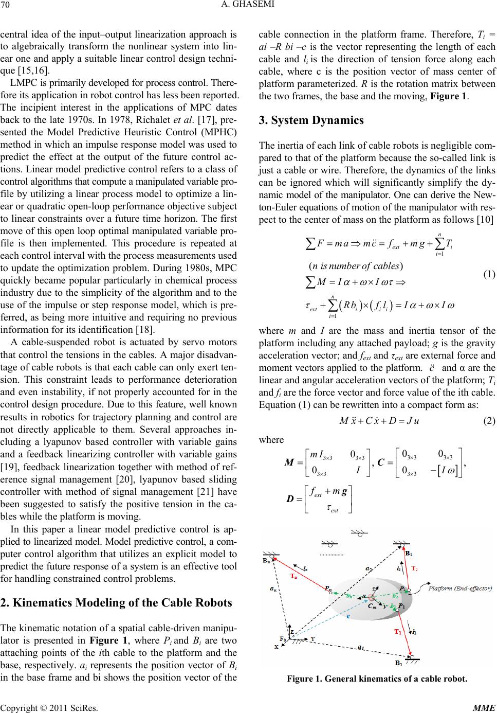

A. GHASEMI
70
central idea of the input–output linearization approach is
to algebraically transform the nonlinear system into lin-
ear one and apply a suitable linear control design techni-
que [15,16].
LMPC is primarily developed for process control. There-
fore its application in robot control has less been reported.
The incipient interest in the applications of MPC dates
back to the late 1970s. In 1978, Richalet et al. [17], pre-
sented the Model Predictive Heuristic Control (MPHC)
method in which an impulse response model was used to
predict the effect at the output of the future control ac-
tions. Linear model predictive control refers to a class of
control algorithms that compute a manipulated variable pro-
file by utilizing a linear process model to optimize a lin-
ear or quadratic open-loop performance objective subject
to linear constraints over a future time horizon. The first
move of this open loop optimal manipulated variable pro-
file is then implemented. This procedure is repeated at
each control interval with the process measurements used
to update the optimization problem. During 1980s, MPC
quickly became popular particularly in chemical process
industry due to the simplicity of the algorithm and to the
use of the impulse or step response model, which is pre-
ferred, as being more intuitive and requiring no previous
information for its identification [18].
A cable-suspended robot is actuated by servo motors
that control the tensions in the cables. A major disadvan-
tage of cable robots is that each cable can only exert ten-
sion. This constraint leads to performance deterioration
and even instability, if not properly accounted for in the
control design procedure. Due to this feature, well known
results in robotics for trajectory planning and control are
not directly applicable to them. Several approaches in-
cluding a lyapunov based controller with variable gains
and a feedback linearizing controller with variable gains
[19], feedback linearization together with method of ref-
erence signal management [20], lyapunov based sliding
controller with method of signal management [21] have
been suggested to satisfy the positive tension in the ca-
bles while the platform is moving.
In this paper a linear model predictive control is ap-
plied to linearized model. Model predictive control, a com-
puter control algorithm that utilizes an explicit model to
predict the future response of a system is an effective tool
for handling constrained control problems.
2. Kinematics Modeling of the Cable Robots
The kinematic notation of a spatial cable-driven manipu-
lator is presented in Figure 1, where Pi and Bi are two
attaching points of the ith cable to the platform and the
base, respectively. ai represents the position vector of Bi
in the base frame and bi shows the position vector of the
cable connection in the platform frame. Therefore, Ti =
ai –R bi –c is the vector representing the length of each
cable and li is the direction of tension force along each
cable, where c is the position vector of mass center of
platform parameterized. R is the rotation matrix between
the two frames, the base and the moving, Figure 1.
3. System Dynamics
The inertia of each link of cable robots is negligible com-
pared to that of the platform because the so-called link is
just a cable or wire. Therefore, the dynamics of the links
can be ignored which will significantly simplify the dy-
namic model of the manipulator. One can derive the New-
ton-Euler equations of motion of the manipulator with res-
pect to the center of mass on the platform as follows [10]

1
1
()
n
ext i
i
n
extii i
i
F
mamc fmgT
nis number ofcables
MI I
Rbf lII
 

 



 






(1)
where m and I are the mass and inertia tensor of the
platform including any attached payload; g is the gravity
acceleration vector; and fext and τext are external force and
moment vectors applied to the platform. and α are the
linear and angular acceleration vectors of the platform; Ti
and fi are the force vector and force value of the ith cable.
Equation (1) can be rewritten into a compact form as:
c

M
xCxD Ju


  (2)
where

33 33
33 33
33 33
00
0,,
00
ext
ext
mI
II
fm









 






MC
g
D
Figure 1. General kinematics of a cable robot.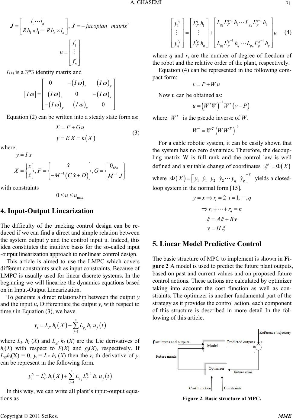

71 A. GHASEMI
1
ll


11
,
nT
nn
jacopian matrix
Rb lRbl






JJ
1
n
f
u
f






I3*3 is a 3*3 identity matrix and



0

 
 
0
0
z
y
z
x
yx
I
II I
II

 








I 




Equation (2) can be written into a steady state form as:
(3)
where

XFGu
yEXhX




6*
11
0
,,
n
x
x
x
XF G
xMCxD
yI
M
J




 
 
  
 
  




with constraints
he difficulty of the tracking control design can be re-
di
between the output y
an
where LF h (X) and Lgj h (X) are the Lie derivatives of
In this way, we can write all plant’s input-output equa-
tio
max
0uu
4. Input-Output Linearization
T
duced if we can find a direct and simple relation between
the system output y and the control input u. Indeed, this
idea constitutes the intuitive basis for the so-called input
-output linearization approach to nonlinear control design.
This article is aimed to use the LMPC which covers
fferent constraints such as input constraints. Because of
LMPC is usually used for linear discrete systems. In the
beginning we will linearize the dynamics equations based
on in Input-Output Linearization.
To generate a direct relationship
d the input u, Differentiate the output yi with respect to
time t in Equation (3), we have
n
 
1j
iF i gij
j
yLhX Lhut



i i
hi(X) with respect to F(X) and gj(X), respectively. If
Lgjhi(X) = 0, yi = LF hi (X) then the ri th derivative of yi
can be represent in the following form.
n
rr r
 
1
1
ii i
j
iF i gFij
j
yLhX LLhut




ns as
11
11
1
1
11
11
11
11
nF
qqq q
FnF
rr
rr
gF g
F
rrr r
qFqgqg q
LL hLL h
yLh
u
yLhLLhLLh



 





 

 









(4)
where q and ri are the number of degree of freedom of
the robot and the relative order of the plant, respectively.
Equation (4) can be represented in the following com-
pact form:
vPWu


Now u can be obtained as

where
:

1
uWWW




vP

W

is the pseudo inverse of W.
For a cable robotic system, it can be easily shown that
th

1
TT
WWWW


e system has no zero dynamics. Therefore, the decoup-
ling matrix W is full rank and the control law is well
defined and a suitable change of coordinates


T
X
 
where

112 2
T
qq
X
yyyyy y





   yiel
loop sy
21,
i
yx ri
ds a closed-
stem in the normal form [15].
,q

 
1q
rr  n
A
Bv
yH





. Linear Model Predictive Control
hown in Fi-
5
he basic structure of MPC to implement is sT
gure 2 A model is used to predict the future plant outputs,
based on past and current values and on proposed future
control actions. These actions are calculated by optimizer
taking into account the cost function as well as con-
straints. The optimizer is another fundamental part of the
strategy as it provides the control action. each component
of this structure is described in more detail In the fol-
lowing of this article.
Figure 2. Basic structure of MPC.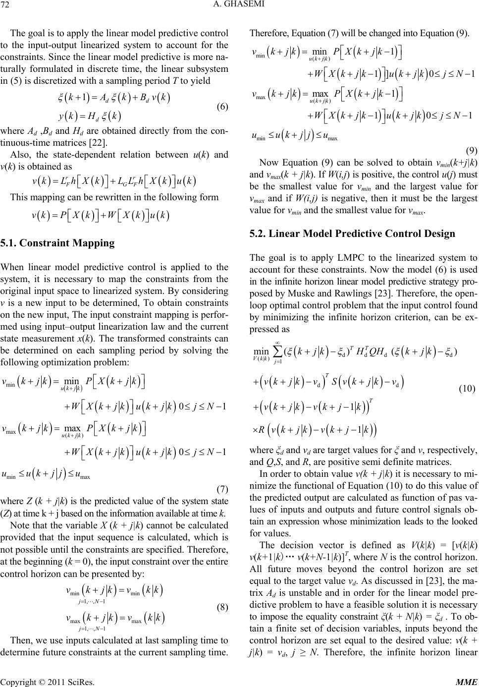

A. GHASEMI
72
The goal tive control
to
is to apply the linear model predic
the input-output linearized system to account for the
constraints. Since the linear model predictive is more na-
turally formulated in discrete time, the linear subsystem
in (5) is discretized with a sampling period T to yield



1kAkBvk   
 
dd
d
yk H k   (6)
where Ad ,Bd and Hd are obtained directly from the con-
t relation between u(k) and
v(
This mapping can be rewritten in the followingrm
.1. Constraint Mapping
hen linear model predictive control is applied to the
tinuous-time matrices [22].
Also, the state-dependen
k) is obtained as

r
vk Lh
 
r
FGF
X kLLhXkuk  
 
fo
 
vkP X kWX kuk

5
W
system, it is necessary to map the constraints from the
original input space to linearized system. By considering
v is a new input to be determined, To obtain constraints
on the new input, The input constraint mapping is perfor-
med using input–output linearization law and the current
state measurement x(k). The transformed constraints can
be determined on each sampling period by solving the
following optimization problem:






 


min
max (|)
min max
01
max
01
uk jk
uk jk
k
WXkjkukjkjN
vkjk PXkjk
WXkjkukjkjN
uukjju





 


 


 


(7)
where Z (k + j|k) is the predicted value of the system s
pr
minvkjk PXkj

 
tate
(Z) at time k + j based on the information available at time k.
Note that the variable X (k + j|k) cannot be calculated
ovided that the input sequence is calculated, which is
not possible until the constraints are specified. Therefore,
at the beginning (k = 0), the input constraint over the entire
control horizon can be presented by:


min min
1, ,1
max max
1, ,1
jN
jN
k
vkjkvkk





(8)
Then, we use inputs calculated at last sampling time to
de
vkjkvk
termine future constraints at the current sampling time.
Therefore, Equation (7) will be changed into Equation (9).





 


min (|)
max (|)
min max
1] 0 1
max 1
101
uk jk
uk jk
W XkjkukjkjN
vkjkPXkjk
WXkjkukjk jN
uukjju




min 1vkjkPXkjk

 

 


 



 


(9)
Now Equation (9) can be solved to obtain vmin(k+
an
.2. Linear Model Predictive Control Design
he goal is to apply LMPC to the linearized system to
j|k)
d vmax(k + j|k). If W(i,j) is positive, the control u(j) must
be the smallest value for vmin and the largest value for
vmax and if W(i,j) is negative, then it must be the largest
value for vmin and the smallest value for vmax.
5
T
account for these constraints. Now the model (6) is used
in the infinite horizon linear model predictive strategy pro-
posed by Muske and Rawlings [23]. Therefore, the open-
loop optimal control problem that the input control found
by minimizing the infinite horizon criterion, can be ex-
pressed as
 
   




ddd d
(|) 1
dd
min ()()
1
1
TT
Vkk j
T
T
kjkHQHkjk
vk jkvSvk jkv
vk jkvk jk
Rvk jkvk jk



 




(10)
where ξd and vd are target values for ξ and v, respectively,
o mi-
ni
sion vector is defined as V(k|k) = [v(k|k)
v(

and Q,S, and R, are positive semi definite matrices.
In order to obtain value v(k + j|k) it is necessary t
mize the functional of Equation (10) to do this value of
the predicted output are calculated as function of pas va-
lues of inputs and outputs and future control signals ob-
tain an expression whose minimization leads to the looked
for values.
The deci
k+1|k) v(k+N-1|k)]T, where N is the control horizon.
All future moves beyond the control horizon are set
equal to the target value vd. As discussed in [23], the ma-
trix Ad is unstable and in order for the linear model pre-
dictive problem to have a feasible solution it is necessary
to impose the equality constraint ξ(k + N|k) = ξd . To ob-
tain a finite set of decision variables, inputs beyond the
control horizon are set equal to the desired value: v(k +
j|k) = vd, j ≥ N. Therefore, the infinite horizon linear

A. GHASEMI
73
model predictive problem Equation (10) can be written
as a finite horizon problem.
12 NN
ddddd
A
BA BB






EE

ddd
0
i
Ni
TT
N
i









   





dd
(|)
1
ddd d
1
dd
1
1
1
T
Vkk
T
NT
j
T
T
SvkNkv
kjkHQHkjk
vk jkvSvk jkv
vk jkvk jk
Rvk jkvk jk
d
K
AHQHA


min 1vkNkv




 
 




(11)
This optimization problem must be solved subjected to
th
 
The solution of Equation (13) belongs to the regular
system. To find the solutions of the tracking one, that of
the regular system should be shifted into the origin of the
system to the steady state described by ξd, and vd. The
desired values must lie within the feasible region defined
by input constraints for linear model predictive control
and minimize the control effort (Equation (15)).
e following constraints:


min min
d
vk
jkvkjkvkjk (12)
Straightforward algebraic manipulation of quadratic
ob
  (13)
where
Equation (13) should be solved subjected to the fol-
lo
 






2
2
min( 0
0
d
T
mm mmds
U
T
mm mmd
ddd
I
UU Q
IUU
Uv 






kNk  
jective function of the corresponding regular system
presented in Equation (11) results in the following stan-
dard quadratic program form:
 
min 2
TT
VHHV V GG 


2*2
:
0
0
0
dd
d
d
d
mm d
subject to
IAB Uy
H
DD UC

 

 



(15)


|1
Vk
kk FFvk
 
Uand Qs are desired value of the input and a positive
definite matrix, respectively. Therefore control law is the
summation of the answers of Equation (13) and Equation
(15) which can be shown in the following form.
1
0
0
,
0
T
dNd
T
dd
S
BK A
FF
BKA













 GG





 



 

(
(
dd d
ukWX kkvkkPXkk
WXkkvkk PXkk




(16)
wing constraints: Figure 3 shows schematic of the proposed structure control.



 
N
d
DD VCC
EE VAk 



(14)
where by considering





max
max
6*
6* min
min
1
,,
1
N
N
vkk
vkNk
I
Ivkk
vkNk





 

 

 


 




DD CC
Figure 3. Schematic of control structure.
0
0

1
2
12
22
12
000
2
2
N
N
TTTTT
dN dddNdddd
TT TT
dN dddNdddd
TNTN T
ddd ddddd
BK ABSBKBRS BAKB
BKA BBKABBKBRS
















HH
2BKBRS BAKBSBAKB

 

A. GHASEMI
74
6. Simulation
In this section, simulation results of applying model pre-
dictive control on a 3D cable robot will be presented.
Table 1. shows the dimensions of the cable robot. We
consider a definite movement of the platform from X0 =
2,.001,–0.001]T to X = [0.2sin(t), 0.4
03t3,0,0,0]T, on a desired trajectory
of Equaqion (10), R = I, Q = I, S = 0.01I, and Qs of
Equation (15), Qs = I.
Since the controller needs platform’s position/orient-
tation, at first, we must solve forward kinematics of the
robot. This has been carried out by the authors using neu-
ral network algorithm [24].
quite well and a trajectory
tra
s of t
Po
[–0.1,–0.1,1.5,0.00
in(t), 1 + 0.2t2 – 0.s
shown in dotted lines by Figures 4(a) to 4(f), for posi-
tion/orientation of the platform.
Also, we consider the parameters of the model predict-
tive controller as: the control horizon N = 25, S, Q, and R
Table 1. Dimension
Position vector X(m) Y(m) Z(m)
Figure 4 shows the model predictive controller with
input-out linearizing worked
cking are done. Figure 5 shows the six tensions in the
cables vs. time. As it can be seen, all of them remain po-
sitive during the motion.
he cable robot.
sition vectorx(m) y(m) z(m)
a1 1.1547 –2 3 b1 –0.2887–0.5 0
a2 1.1547 –2 3
a 1.1547 2 3
b2 0.5774 0 0
3b3 0.5774 0 0
a4 1.1547 870.5 0
a –2.309 0 3 b –0.28870.5 0
–
2 3 b4 –0.28
5
a6
5
b6 –2.309 0 3 0.2887-0.5 0
(a) (b)
(c) (d)
(e) (f)
Figure 4. Plots of desired and actual position and orientation of the platform, (a)-(c) position in X-Y-Z directions, respectively,
(d)-(f) orientation around X-Y-Z direction, respectively.

75 A. GHASEMI
(a) (b)
(c) (d)
(e) (f)
7. Conclusions
In this paper, a linear model predictive controller toge-
ther with an input-output linearizing control strategy for
a constrained robotic system, a 3D cable robot, was de-
veloped and evaluated. The control system is comprised
of: 1) an input-output linearizing controller that accounts for
cable robot nonlinearities; 2) a constraint mapping sche-
e that transforms the actual input
onstraints on the feedback linearized sy
near model predictive controller that provides explicit
nput constraints. The simulation re-
ectiveness of the proposed method. It
Figure 5. Plots of tension trajectories.
m
c
constraints into input
stem; and 3) a
li
compensation for i
ults showed the effs
is worth nothing that this approach can be extended for
the redundant cable robots.
8. References
[1] D. Stewart, “A Platform with Six Degrees of Freedom,”
Proceedings of the Institution of Mechanical Engineer, Vol.
180, No. 15, 1965, pp. 371-386.
doi:10.1243/PIME_PROC_1965_180_029_02
[2] J. -P. Merlet, “Parallel Robots, Solid Mechanics and Its
2006, pp. 890-902.
[7] A. T. Riechel and I. Ebert-Uphoff, “Force-Feasible Work-
space Analysis for Underconstrained Pointmass Cable
Robots,” Proceedings of I
Applications,” Kluwer, Norwell, 2001.
[3] J. -P. Merlet, “Still a Long Way to Go on the Road for
Parallel Mechanisms,” A Keynote Speech at Design En-
gineering Technical Conferences, Montreal, 29 Septem-
ber-2 October 2002.
[4] J. -P. Merlet, “Parallel Robots, Open Problems,” INRIA
Sophia-Antipolis, France. http://www.-sop.inria.fr
[5] L. -W. Tsai, “Robot Analysis, The Mechanics of Serial and
rs,” Wiley, New York, 1999.
A. T. Riechel and I. Ebert-Uphoff, “Wrench-
rkspace Generation for Cabledriven Robots,”
Journal of Intelligent and Robotic Systems, Vol. 22, No. 4,
EEE International Conference on
Robotics and Automation, New Orleans, 26 April-1 May
4962.
W. Choe, S. Tanaka and S. R. Pandian,
[9] P. Lafourcade, M. Llibre and C. Reboulet, “Design of a Par-
Parallel Manipulato
[6] P. Bosscher,
Feasible Wo
2004, pp. 4956-
]S. Kawamura,[8
“Development of an Ultrahigh Speed FALCON Using
Wire Drive System,” In Proceedings of the 1995 IEEE
International Conference on Robotics and Automation,
21-27 May 2003, pp. 215-220.

A. GHASEMI
76
mental Issues and
plication of HIL Microgravity Con-
allel Wire-Driven Manipulator for Wind Tunnels,” In
Proceedings of the Workshop on Funda
Future Research Directions for Parallel Mechanisms and
Manipulators, Quebec, 3-4 October 2002, pp. 187-194.
[10] X. Diao, O. Ma and R. Paz, “Study of 6-DOF Cable Ro-
bots for Potential Ap
tact-Dynamics Simulation,” In Proceedings of the AIAA
Modeling and Simulation Technologies Conference and
Exhibit, Keystone, 21-24 August 2006, pp. 1097-1110.
[11] P. Gallina, G. Rosati and A. Rossi, “3-D.O.F. Wire Driven
Planar Haptic Interface,” Journal of Intelligent and Ro-
botic Systems,Vol. 32, No. 1, 2001, pp. 23-36.
doi:10.1023/A:1012095609866
[12] J. Albus, R. Bostelman and N. Dagalakis, “The NIST
Robocrane,” Journal of Robotic Systems, Vol. 10, No. 5,
1993, pp. 709-724. doi:10.1002/rob.4620100509
[13] Y. Q. Zheng, “Workspace Analysis of a Six DOF Wire-
Driven Parallel Manipulator,” Proceedings of the WORK-
SHOP on Fundamental Issues and Future Research De-
rection for Parallel Mechanisms and Manipulators, Que-
bec, 3-4 October 2002, pp. 287-293.
[14] W. J. Shiang, D. Cannon and J. Gorman, “Dynamic
Analysis of the Cable Array Robotic Crane,” Proceedings
of the IEEE International Conference on Robotics and
Automation, Detroit, 10-15 May 1999, pp. 2495-2500.
[15] J. J. Slotine and W. Leiping, “Applied Nonlinear Control,”
Prentice Hall, Englewood Cliffs, 1991.
[16] H. Khalil, “Nonlinear Systems,” 3rd Edition, Prentice-Hall,
Upper Saddle River, 2002.
[17] J. Richalet, A. Raault, J. L. Testud and J. Papon, “Model
Predictive Heuristic Control: A pplication to Industry
Processes,” Automatica, Vol. 14. No. 2, 1978, pp. 413-428.
doi:10.1016/0005-1098(78)90001-8
[18] C. E. Garcia, D. M. Prett and Morari, “Model Predictive
Control: Theory and Practice—a Survey,” Automatica,
Vol. 25, No. 3 1989, pp. 335-348.
doi:10.1016/0005-1098(89)90002-2
[19] A. B. Alp and A. K. Agrawal, “Cable Suspended Robots:
ce on Robotics and
Design, Planning and Control,” International Conference
on Robotics Robotics & Automation, Washington, DC, 9-
13 May 2002, pp. 556-561.
[20] S. R. Oh and A. K. Agrawal, “Controller Design for a
Non-redundant Cable Robot Under Input Constraint,” ASME
International Mechanical Engineering Congress & Expo-
sition, 16-21 November 2003, Washington, DC.
[21] S. R. Oh and A. K. Agrawal, “A Control Lyapunov Ap-
proach for Feedback Control of Cable-Suspended Ro-
bots,” IEEE International Conferen
Automation, 10-14 April 2007, pp. 4544-4549.
[22] F. Franklin, J. Powell and L. Workman “Digital Control
of Dynamic Systems” 2nd Edition, Addison Wesley, Bos-
ton, 1994, pp. 40-70.
[23] K. R. Muske and J. B. Rawlings, “Model predictive con-
trol with linear models,” AIChE Journal, Vol. 39, No. 2,
1993, pp. 262-287. doi:10.1002/aic.690390208
[24] A. Ghasemi, M. Eghtesad and M. Farid “Neural Network
Solution for Forward Kinematics Problem of Cable Ro-
bot,” Journal of Intelligent and Robotic Systems, Vol. 60,
No. 2, 2010, pp. 201-215.
doi:10.1007/s10846-010-9421-z