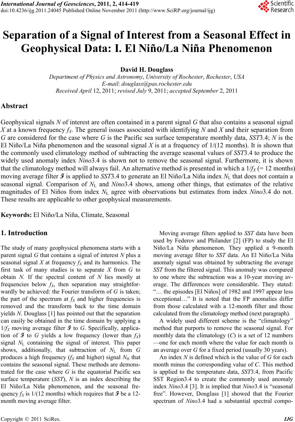International Journal of Geosciences, 2011, 2, 414-419
doi:10.4236/ijg.2011.24045 Published Online November 2011 (http://www.SciRP.org/journal/ijg)
Separation of a Signal of Interest from a Seasonal Effect in
Geophysical Data: I. El Niño/La Niña Phenomenon
David H. Douglass
Department of Physics and Astronomy, University of Rochester, Rochester, USA
Received April 12, 2011; revised July 9, 2011; accepted September 2, 2011
Abstract
Geophysical signals N of interest are often contained in a parent signal G that also contains a seasonal signal
X at a known frequency fX. The general issues associated with identifying N and X and their separation from
G are considered for the case where G is the Pacific sea surface temperature monthly data, SST 3.4; N is the
El Niño/La Niña phenomenon and the seasonal signal X is at a frequency of 1/(12 months). It is shown that
the commonly used climatology method of subtracting the average seasonal values of SST3.4 to produce the
widely used anomaly index Nino3.4 is shown not to remove the seasonal signal. Furthermore, it is shown
that the climatology method will always fail. An alternative method is presented in which a 1/fX (= 12 months)
moving average filter F is applied to SST3.4 to generate an El Niño/La Niña index NL that does not contain a
seasonal signal. Comparison of NL and Nino3.4 shows, among other things, that estimates of the relative
magnitudes of El Niños from index NL agree with observations but estimates from index Nino3.4 do not.
These results are applicable to other geophysical measurements.
Keywords: El Niño/La Niña, Climate, Seasonal
1. Introduction
The study of many geophysical phenomena starts with a
parent signal G that contains a signal of interest N plus a
seasonal signal X at frequency fX and its harmonics. The
first task of many studies is to separate X from G to
obtain N. If the spectral content of N lies mostly at
frequencies below fX, then separation may straightfor-
wardly be achieved: the Fourier transform of G is taken;
the part of the spectrum at fX and higher frequencies is
removed and the transform back to the time domain
yields N. Douglass [1] has pointed out that the separation
can easily be obtained in the time domain by applying a
1/fX moving average filter F to G. Specifically, applica-
tion of F to G yields a low frequency (lower than fX)
signal NL containing the signal of interest. This paper
shows, additionally, that subtraction of NL from G
produces a high frequency (fX and higher) signal NH that
contains the seasonal signal. These methods are demons-
trated for the case where G is the equatorial Pacific sea
surface temperature (SST), N is an index describing the
El Niño/La Niña phenomenon, and the seasonal fre-
quency fX is 1/(12 months) which requires that F be a 12-
month moving average filter.
Moving average filters applied to SST data have been
used by Federov and Philander [2] (FP) to study the El
Niño/La Niña phenomenon. They applied a 9-month
moving average filter to SST data. An El Niño/La Niña
anomaly signal was obtained by subtracting the average
SST from the filtered signal. This anomaly was compared
to one where the subtraction was a 10-year moving av-
erage. The differences were considerable. They stated:
“… the episodes [El Niños] of 1982 and 1997 appear less
exceptional…” It is noted that the FP anomalies differ
from those calculated with a 12-month filter and those
calculated from the climatology method (next paragraph).
A widely used different scheme is the “climatology”
method that purports to remove the seasonal signal. For
monthly data the climatology (C) is a set of 12 numbers
—one for each month where the value for each month is
an average over G for a fixed period (usually 30 years).
An index N is defined which is the value of G for each
month minus the corresponding value of C. This method
is applied to the temperature data, SST3.4, from Pacific
SST Region3.4 to create the commonly used anomaly
index Nino3.4 [3]. It is implied that Nino3.4 is “seasonal
free”. However, Douglass [1] showed that the Fourier
spectrum of Nino3.4 had a substantial spectral compo-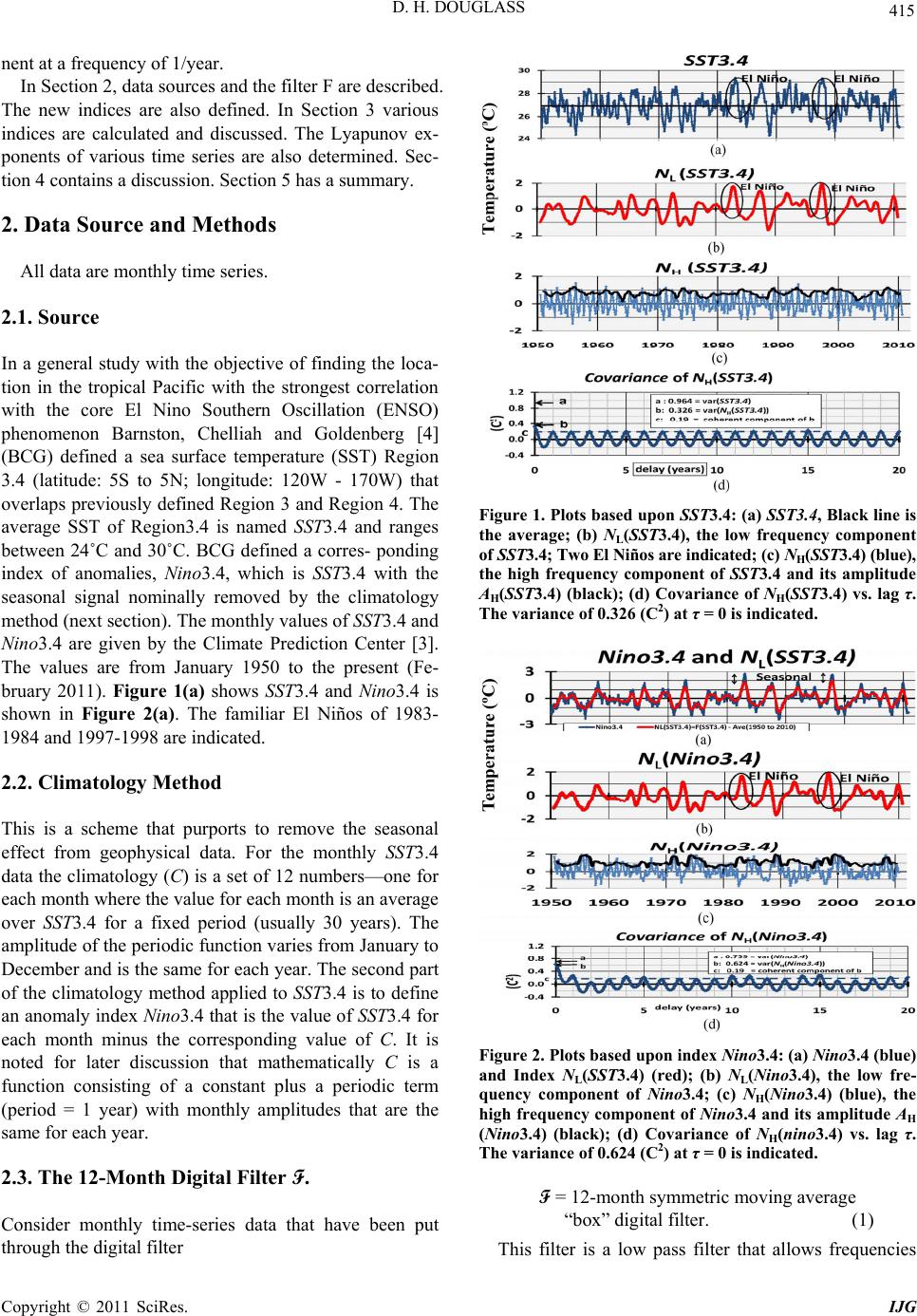

D. H. DOUGLASS
415
nent at a frequency of 1/year.
In Section 2, data sources and the filter F are described.
The new indices are also defined. In Section 3 various
indices are calculated and discussed. The Lyapunov ex-
ponents of various time series are also determined. Sec-
tion 4 contains a discussion. Section 5 has a summary.
2. Data Source and Methods
All data are monthly time series.
2.1. Source
In a general study with the objective of finding the loca-
tion in the tropical Pacific with the strongest correlation
with the core El Nino Southern Oscillation (ENSO)
phenomenon Barnston, Chelliah and Goldenberg [4]
(BCG) defined a sea surface temperature (SST) Region
3.4 (latitude: 5S to 5N; longitude: 120W - 170W) that
overlaps previously defined Region 3 and Region 4. The
average SST of Region3.4 is named SST3.4 and ranges
between 24˚C and 30˚C. BCG defined a corres- ponding
index of anomalies, Nino3.4, which is SST3.4 with the
seasonal signal nominally removed by the climatology
method (next section). The monthly values of SST3.4 and
Nino3.4 are given by the Climate Prediction Center [3].
The values are from January 1950 to the present (Fe-
bruary 2011). Figure 1(a) shows SS T3.4 and Nino3.4 is
shown in Figure 2(a). The familiar El Niños of 1983-
1984 and 1997-1998 are indicated.
2.2. Climatology Method
This is a scheme that purports to remove the seasonal
effect from geophysical data. For the monthly SST3.4
data the climatology (C) is a set of 12 numbers—one for
each month where the value for each month is an average
over SST3.4 for a fixed period (usually 30 years). The
amplitude of the periodic function varies from January to
December and is the same for each year. The second part
of the climatology method applied to SST3.4 is to define
an anomaly index Nino3.4 that is the value of SST3.4 for
each month minus the corresponding value of C. It is
noted for later discussion that mathematically C is a
function consisting of a constant plus a periodic term
(period = 1 year) with monthly amplitudes that are the
same for each year.
2.3. The 12-Month Digital Filter F.
Consider monthly time-series data that have been put
through the digital filter
Figure 1. Plots based upon SST3.4: (a) SST3.4, Black line is
the average; (b) N
L(SST3.4), the low frequency component
of SST3.4; Two El Niños are indicated; (c) NH(SST3.4) (blue),
the high frequency component of SST3.4 and its amplitude
AH(SST3.4) (black); (d) Covariance of NH(SST3.4) vs. lag τ.
The variance of 0.326 (C2) at τ = 0 is indicated.
Figure 2. Plots based upon index Nino3.4: (a) Nino3.4 (blue)
and Index NL(SST3.4) (red); (b) NL(Nino3.4), the low fre-
quency component of Nino3.4; (c) NH(Nino3.4) (blue), the
high frequency component of Nino3.4 and its amplitude AH
(Nino3.4) (black); (d) Covariance of NH(nino3.4) vs. lag τ.
The variance of 0.624 (C2) at τ = 0 is indicated.
F = 12-month symmetric moving average
“box” digital filter. (1)
This filter is a low pass filter that allows frequencies

D. H. DOUGLASS
416
lower than (1/12) month–1 to pass with only slight atte-
nuation. This filter has an additional important property
that is not generally recognized. The Fourier transform of
F is



12 () sinπ12sin π
H
fff, which has zeros at
multiples of the frequency f = (1/12) month–1 [5]. Thus,
signals whose frequencies are exactly f = (1/12) month–1
and its harmonics are removed. This second property is
highly desirable in reducing an unwanted seasonal signal
that contains an annual component and its harmonics.
One frequently sees the use of k-month filters where k
has values 3, 5, 7, 9, 11, 12, 13 in attempts to reduce the
seasonal signal; the k = 12 filter is obviously best for
removal of such a signal. Because the center of this
filter is between time series data points, one has to place
the center of the filter one half interval before or after the
reference data point. Here, the choice is “after”. The 12-
month filter is then described as “6-1-5”, where “1” is
the reference. There is a loss of six data points at the
beginning of the time series and five at end of the time-
series.
2.4. Climate Indices
The filter F is applied to a time series G to create a “low
frequency” index NL,
NL(G) = F(G) – average F(G), (2)
where the average is over a range of G (1981-2010 in
this paper) and a “high frequency” index
NH(G) = G – F(G). (3)
Equation (2) been applied to SST3.4 data by Douglass
[1] to define a new El Niño/La Niña index NL(SST3.4).
This is shown in Figure 1(b). Application of Equation (3)
to SST3.4 creates NH(SST3.4), which contains the seaso-
nal signal. NH(SST3.4) is plotted in Figure 1(c), which
shows a strong periodicity of one year. The amplitude of
NH is defined as

1/2
HH
2
A
RMS N, (4)
where RMS is the square root of the symmetric 12-
month mean square of NH. AH of NL(SST3.4) is shown in
Figure 1(c) (black).
The variously defined quantities are listed in Table 1.
2.5. Covariance
The covariance (cov ar) of a signal x(t) is defined as
  
1
1
covar var
1
K
x
xt xtx
K

 
; (5)
where t is a time lag; the summation is over the equally
spaced values of x; var(x) is the usual statistical variance
Table 1. Definitions of various quantities.
Definitions
G A geophysical time series that contains a signal N of interest plus a
seasonal signal of known period.
SST3.4 is an example which contains the El Niño/La
Niña phenomenon plus a seasonal signal of period
12-months.
Filter F n-month symmetric moving average “box” digital filter. n = 12 for SST3.4Used to create the two indices in the next two rows.
NL(G) NL = F(G) – average F(G) This is the “low frequency” component of G.
NH(G) NH = T – F(G) This is the “high frequency” component of G.
AH(G) AH = 21/2RMS(NH) Amplitude of NH.
Region 3.4 Area in central Equatorial Pacific [5S to 5N; 120W to 170W] A primary reference area for El Niño/La Niña
phenomenon.
SST3.4 Monthly values of the average Sea Surface Temperature (SST) over
region 3.4.
Ranges between 24˚C and 30˚C. Consists of the El
Niño/La Niña phenomenon plus a seasonal effect of
1-year period.
Climatology For monthly data the Climatology (C) is a set of 12 constant numbers that
are an average of G for each month over a fixed period (usually 30 years).
Used in the construction of the index of anomalies such
as Nino3.4.
Nino3.4 The commonly used index of anomalies that is defined as SST3.4 minus CIt is stated that the seasonal effect has been “removed”.
The text explains that this is not true.
Chaotic Properties of a Dynamic System
Lyapunov exponents Comments
At least one exponent > 0.
Sum of exponents < 0.
Sum < 0 means dissipative dynamics.
The signal is “well-defined”.
At least one exponent > 0.
Sum of exponents > 0 The signal is “ill-defined”.

D. H. DOUGLASS
417
and r(t) is the commonly used delayed Pearson autocor-
relation function. When t = 0, covar(0) = var(x). For later
reference it is noted that if x is a random variable, there is
very little covariance after t = 0.
3. Analysis
The average, variance and trend of various time series
from SST3.4 were calculated and are listed in Table 2(a).
Also listed are the magnitudes of the El Niños of 1982-
1983 and 1997-1998 according to several different in-
dices.
Index NL was computed for SST3.4 and is shown in
Figure 1(b). The seasonal signal NH(SST3.4) and its
amplitude A
H(SST3.4) are shown in Figure 1(c). Of
particular interest is the covariance of NH(SST3.4) vs. lag
t shown in Figure 1(d). For large lags, the covariance of
NH (SS T3.4) shows periodic behavior at a period of 1
year of amplitude 0.20 C2 which indicates a sustained
oscillation almost certainly of solar origin. Computation
of the average value for each month of NH (SS T3.4)
shows that the maximum (0.75 C) occurs during Apr/
May and that a broad minimum (–0.43 C) occurs during
Dec/Jan. The covariance of NH(SST3.4) at t = 0 is the
variance whose value is 0.326 C2. Since the variance of
Table 2. (a) Statistical and other properties of SST3.4 and
Niño3.4; (b) Variances.
(a)
Statistical and other properties
SST3.4 Nino3.4
SST3.4 NL NH Nino3.4 NL NH
Average (C)
(1950-2010) 26.942 0.000 0.003 –0.096 –0.0810.083
Variance (C2)
(1950-2010) 0.964 0.458 (Note A)0.326 0.759 0.458 (Note A)0.624
Slope (C/decade)
(1950-2010) 0.043 0.045 0.003 0.044 0.045–0.042
Amplitude El Niño
of 1982-1983 (C) 1.78 2.79
Amplitude El Niño
of 1997-1998 (C) 1.98 2.69
Note A. These two values are very close. The 12 climatology values used to
calculate Nin o3.4 are: 26.6, 26.7, 27.2, 27.8, 27.9, 27.7, 27.2 26.8, 26.7,
26.7, 26.7, and 26.6 (C).
(b)
Comparison of variances (C2)
SST3.4 Nino3.4
Parent 0.964 0.759
NH 0.326 0.624
NH_randoma ≈ 0.13 ≈ 0.43
NH_coherenta ≈ 0.20 ≈ 0.19
Note a. The random component of the variance is the amount of the abrupt
drop in covar(0). The rest of covar(0) is the coherent component.
the coherent signal is 0.20 C2, then the difference from
0.326 C2 of ~0.19 C2 can be inferred to be due to random
processes. The variance of the parent signal, SST3.4 of
0.964 C2 is also indicated on the plot. Thus, SST3.4
contains a seasonal signal whose variance is about 1/3 of
that of SST3.4. The seasonal signal consists of two com-
ponents whose variances are: a coherent signal at a
period of 1 year (variance = 0.20 C2) and a random
signal (variance = 0.13 C2).
The same calculations were carried out on index
Nino3.4 and are shown in Figures 2(a-d). What is the
effect of using the climatology to produce index Nino3.4?
The variance of Nino3.4 is 0.749 C2 which is less than
the 0.964 C2 value of SST3.4. However, the variance of
the seasonal signal, NH(Nino3.4), is 0.624 C2. Thus, not
only is the variance of the seasonal signal not reduced by
the climatology method but it is now nearly twice in
magnitude! This “not removed” seasonal signal consists
of two components whose variances are: a coherent
signal at a period of 1 year (variance = 0.19 C2) and a
random signal (variance = 0.43 C2). The climatology
method has increased the random component of the
seasonal signal while keeping the coherent component
nearly the same. In sum, the climatology method does
not remove the seasonal signal from SST3.4.
4. Discussion
4.1. Separation of the Seasonal Signal
One of the main conclusions of this study is that the
“season free” index Nino3.4 contains a substantial com-
ponent of a seasonal signal. Thus the climatology method
fails. Furthermore, no set of climatology values will
remove the seasonal signal from SST3.4. This is because
the climatology is a function consisting of a constant plus
a periodic function with monthly amplitudes that are the
same for each year while the seasonal signal NH calcu-
lated from the SST3.4 data (See Figure 1(c)) is also a
periodic function the amplitude is not a constant. Thus,
the climatology method subtracts an incorrect periodic
signal from the parent SST3.4 signal and has produced a
different seasonal signal that is larger than it was before.
Somewhat miraculously, the filter F applied to Nino3.4
will remove both the incorrect seasonal function intro-
duced by the climatology method and the original seaso-
nal signal. So NL(Nino3.4) ≈ N
L(SST3.4), which agrees
with the observation of Douglass [1].
It is important to know the extent to which Nino3.4 is
“contaminated” by a seasonal signal because this index is
widely used. For example, the United States National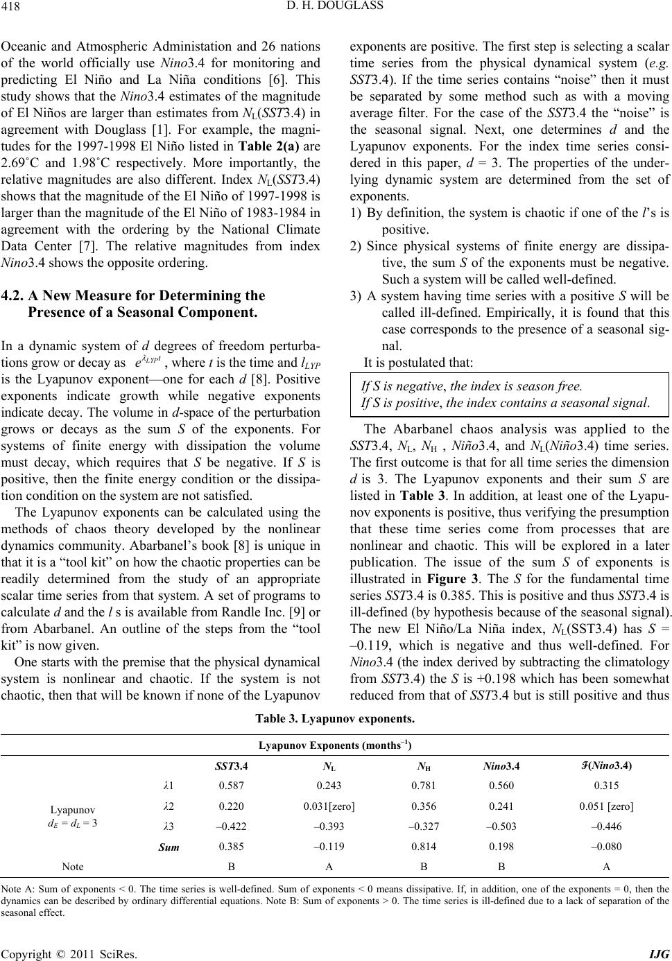

D. H. DOUGLASS
418
Oceanic and Atmospheric Administation and 26 nations
of the world officially use Nino3.4 for monitoring and
predicting El Niño and La Niña conditions [6]. This
study shows that the Nino3.4 estimates of the magnitude
of El Niños are larger than estimates from NL(SST3.4) in
agreement with Douglass [1]. For example, the magni-
tudes for the 1997-1998 El Niño listed in Table 2(a) are
2.69˚C and 1.98˚C respectively. More importantly, the
relative magnitudes are also different. Index NL(SST3.4)
shows that the magnitude of the El Niño of 1997-1998 is
larger than the magnitude of the El Niño of 1983-1984 in
agreement with the ordering by the National Climate
Data Center [7]. The relative magnitudes from index
Nino3.4 shows the opposite ordering.
4.2. A New Measure for Determining the
Presence of a Seasonal Component.
In a dynamic system of d degrees of freedom perturba-
tions grow or decay as
L
YPt
e

, where t is the time and lLYP
is the Lyapunov exponent—one for each d [8]. Positive
exponents indicate growth while negative exponents
indicate decay. The volume in d-space of the perturbation
grows or decays as the sum S of the exponents. For
systems of finite energy with dissipation the volume
must decay, which requires that S be negative. If S is
positive, then the finite energy condition or the dissipa-
tion condition on the system are not satisfied.
The Lyapunov exponents can be calculated using the
methods of chaos theory developed by the nonlinear
dynamics community. Abarbanel’s book [8] is unique in
that it is a “tool kit” on how the chaotic properties can be
readily determined from the study of an appropriate
scalar time series from that system. A set of programs to
calculate d and the l s is available from Randle Inc. [9] or
from Abarbanel. An outline of the steps from the “tool
kit” is now given.
One starts with the premise that the physical dynamical
system is nonlinear and chaotic. If the system is not
chaotic, then that will be known if none of the Lyapunov
exponents are positive. The first step is selecting a scalar
time series from the physical dynamical system (e.g.
SST3.4). If the time series contains “noise” then it must
be separated by some method such as with a moving
average filter. For the case of the SST3.4 the “noise” is
the seasonal signal. Next, one determines d and the
Lyapunov exponents. For the index time series consi-
dered in this paper, d = 3. The properties of the under-
lying dynamic system are determined from the set of
exponents.
1) By definition, the system is chaotic if one of the l’s is
positive.
2) Since physical systems of finite energy are dissipa-
tive, the sum S of the exponents must be negative.
Such a system will be called well-defined.
3) A system having time series with a positive S will be
called ill-defined. Empirically, it is found that this
case corresponds to the presence of a seasonal sig-
nal.
It is postulated that:
The Abarbanel chaos analysis was applied to the
SST3.4, NL, NH , Niño3.4, and NL(Niño3.4) time series.
The first outcome is that for all time series the dimension
d is 3. The Lyapunov exponents and their sum S are
listed in Table 3. In addition, at least one of the Lyapu-
nov exponents is positive, thus verifying the presumption
that these time series come from processes that are
nonlinear and chaotic. This will be explored in a later
publication. The issue of the sum S of exponents is
illustrated in Figure 3. The S for the fundamental time
series SST3.4 is 0.385. This is positive and thus SST3.4 is
ill-defined (by hypothesis because of the seasonal signal).
The new El Niño/La Niña index, NL(SST3.4) has S =
–0.119, which is negative and thus well-defined. For
Nino3.4 (the index derived by subtracting the climatology
from SST3.4) the S is +0.198 which has been somewhat
reduced from that of SST3.4 but is still positive and thus
Table 3. Lyapunov exponents.
Lyapunov Exponents (months–1)
SST3.4 NL NH Nino3.4 F(Nino3.4)
λ1 0.587 0.243 0.781 0.560 0.315
λ2 0.220 0.031[zero] 0.356 0.241 0.051 [zero]
λ3 –0.422 –0.393 –0.327 –0.503 –0.446
Lyapunov
dE = dL = 3
Sum 0.385 –0.119 0.814 0.198 –0.080
Note B A B B A
Note A: Sum of exponents < 0. The time series is well-defined. Sum of exponents < 0 means dissipative. If, in addition, one of the exponents = 0, then the
dynamics can be described by ordinary differential equations. Note B: Sum of exponents > 0. The time series is ill-defined due to a lack of separation of the
seasonal effect.
If S is negative, the index is season free.
If S is positive, the index contains a seasonal signal.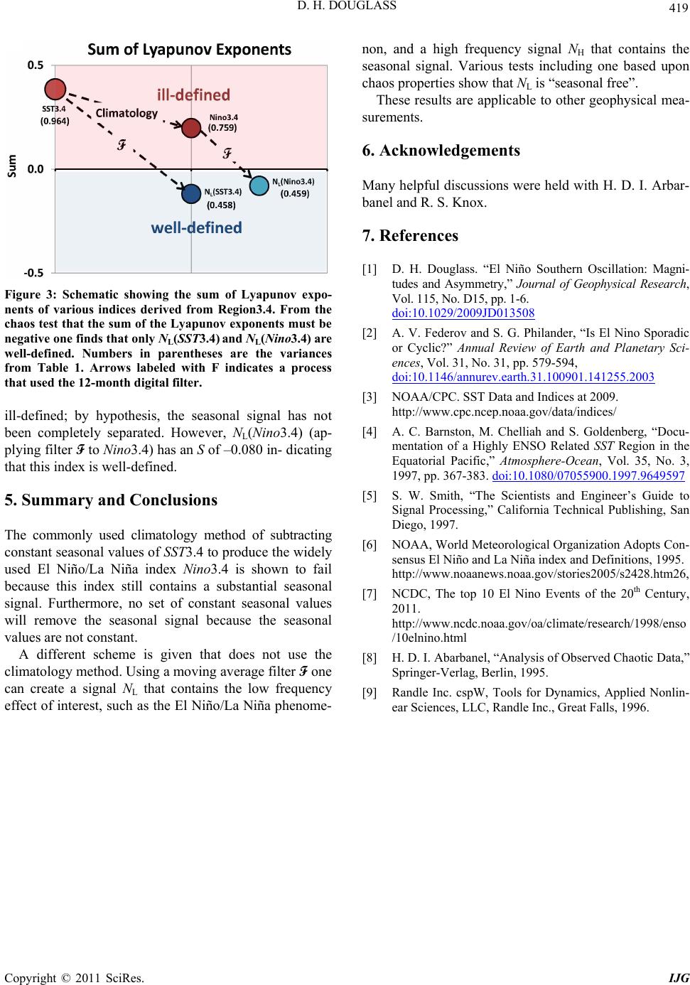

D. H. DOUGLASS
419
Figure 3: Schematic showing the sum of Lyapunov expo-
nents of various indices derived from Region3.4. From the
chaos test that the sum of the Lyapunov exponents must be
negative one finds that only NL(SST3.4) and NL(Nino3.4) are
well-defined. Numbers in parentheses are the variances
from Table 1. Arrows labeled with F indicates a process
that used the 12-month digital filter.
ill-defined; by hypothesis, the seasonal signal has not
been completely separated. However, NL(Nino3.4) (ap-
plying filter F to Nino3.4) has an S of –0.080 in- dicating
that this index is well-defined.
5. Summary and Conclusions
The commonly used climatology method of subtracting
constant seasonal values of SST3.4 to produce the widely
used El Niño/La Niña index Nino3.4 is shown to fail
because this index still contains a substantial seasonal
signal. Furthermore, no set of constant seasonal values
will remove the seasonal signal because the seasonal
values are not constant.
A different scheme is given that does not use the
climatology method. Using a moving average filter F one
can create a signal NL that contains the low frequency
effect of interest, such as the El Niño/La Niña phenome-
non, and a high frequency signal NH that contains the
seasonal signal. Various tests including one based upon
chaos properties show that NL is “seasonal free”.
These results are applicable to other geophysical mea-
surements.
6. Acknowledgements
Many helpful discussions were held with H. D. I. Arbar-
banel and R. S. Knox.
7. References
[1] D. H. Douglass. “El Niño Southern Oscillation: Magni-
tudes and Asymmetry,” Journal of Geophysical Research,
Vol. 115, No. D15, pp. 1-6.
doi:10.1029/2009JD013508
[2] A. V. Federov and S. G. Philander, “Is El Nino Sporadic
or Cyclic?” Annual Review of Earth and Planetary Sci-
ences, Vol. 31, No. 31, pp. 579-594,
doi:10.1146/annurev.earth.31.100901.141255.2003
[3] NOAA/CPC. SST Data and Indices at 2009.
http://www.cpc.ncep.noaa.gov/data/indices/
[4] A. C. Barnston, M. Chelliah and S. Goldenberg, “Docu-
mentation of a Highly ENSO Related SST Region in the
Equatorial Pacific,” Atmosphere-Ocean, Vol. 35, No. 3,
1997, pp. 367-383. doi:10.1080/07055900.1997.9649597
[5] S. W. Smith, “The Scientists and Engineer’s Guide to
Signal Processing,” California Technical Publishing, San
Diego, 1997.
[6] NOAA, World Meteorological Organization Adopts Con-
sensus El Niño and La Niña index and Definitions, 1995.
http://www.noaanews.noaa.gov/stories2005/s2428.htm26,
[7] NCDC, The top 10 El Nino Events of the 20th Century,
2011.
http://www.ncdc.noaa.gov/oa/climate/research/1998/enso
/10elnino.html
[8] H. D. I. Abarbanel, “Analysis of Observed Chaotic Data,”
Springer-Verlag, Berlin, 1995.
[9] Randle Inc. cspW, Tools for Dynamics, Applied Nonlin-
ear Sciences, LLC, Randle Inc., Great Falls, 1996.