Applied Mathematics, 2011, 2, 1378-1381
doi:10.4236/am.2011.211194 Published Online November 2011 (http://www.SciRP.org/journal/am)
Biorthogonal Wavelet Based Algebraic Multigrid
Preconditioners for Large Sparse Linear Systems
A. Padmanabha Reddy, Nagendrappa M. Bujurke*
Department of Mat hematics, Karnatak University, Dharwad, India
Received June 24, 201 1; revised July 23, 2011; accepted August 1, 2011
Abstract
In this article algebraic multigrid as preconditioners are designed, with biorthogonal wavelets, as intergrid
operators for the Krylov subspace iterative methods. Construction of hierarchy of matrices in algebraic mul-
tigrid context is based on lowpass filter version of Wavelet Transform. The robustness and efficiency of this
new approach is tested by applying it to large sparse, unsymmetric and ill-conditioned matrices from Tim
Davis collection of sparse matrices. Proposed preconditioners have potential in reducing cputime, operator
complexity and storage space of algebraic multigrid V-cycle and meet the desired accuracy of solution com-
pared with that of orthogonal wavelets.
Keywords: Algebraic Multigrid, Preconditioner, Wavelet Transform, Sparse Matrix, Krylov Subspace
Iterative Methods
1. Introduction
The linear system of algebraic equations
A
xb

(1.1)
where
A
is non-singular matrix and b is vector
of size n arise while discretising various equations using
finite difference, finite element and domain decomposi-
tion schemes etc.
nn
One of the useful schemes to solve (1.1) is multigrid.
For multigrid (geometric/algebraic), if one has used the
proper smoother, restriction and prolongation operators,
then the multigrid algorithm will require so few cycles to
reach the level of truncation error. But unfortunately
such operators are not always known for all problems. In
such cases, acceleration of Krylov subspace iterative me-
thods will help. Equiv alently, one can also cons ider mul-
tigrid as a preocnditioner for one of the Krylov subspace
iterative methods [1].
In classical schemes, designing/constructing a suitable
preconditioner for unstructured matrix
A
-arising from
nonsmooth region or mesh free type problems is an im-
possible/tough task. Furthermore, Algebraic multigrid-a
general purpose purely algebraic scheme which relays
only on the elements of
A
and works as universal pre-
conditioner heralds a cutting edge of current research on
preconditioners.
Orthogonal (Daubechies) wavelet based precondition-
ers are developed for various types of large sparse ma-
trices [2-4]. Kumar and Mehra [2] developed matrix
splitting based preconditioners, where as in [3] and [4]
wavelet based algebraic multigrid as preconditioners for
Krylov subspace iterative methods are developed. In
these articles authors have shown that wavelet based
algorithms are efficient and robust compared with that of
classical schemes such as matrix splitting, algebraic mul-
tigrid and incomplete LU factorization(ilu) based precon-
ditioners for Krylov subspace iterative methods. These
studies motivate us to develop biorthogonal wavelet based
preconditioners for Krylov subspace iterative methods.
2. Discrete Biorthogonal Wavelet Transform
For a given ,pp


p

(,)pp

, such that is even, there
exists compactly supported biorthogonal spline wavelets
of order called Cohen Daubechies Feauveau wave-
lets (CDF) which form biorthogonal bases for
pp
,p


2
LR
Ws
[5]. Let be a vector (signal) of length , its
one level biorthogonal wavelet transform is given by
. For CDF
sn


2,2 , its wavelet tran sform matrix is

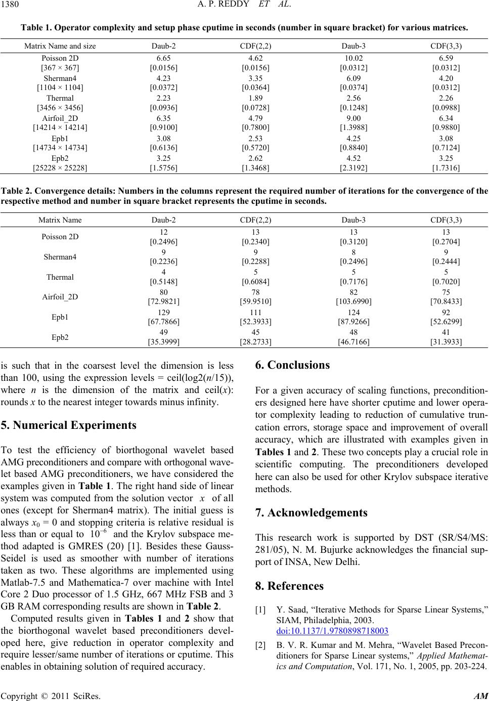
A. P. REDDY ET AL.1379
01
101
101
01123
10123
101
2
22 nn
hh
hhh
hhh
gg gg g
ggggg
ggg

























 



W






Matrix W contains first 2n rows which are lowpass
filter coefficients and remaining 2nrows are highpass
filter coefficients. W can be derived for various
by symmetric extension of filters [6] and is any
natural number [3]. Here first half of is a represen-
tation of s at a lower resolution level. This represen tation
has to preserve average, first moment and so on of the
original signal s. Preservation of these moments depends
on the accuracy of the scaling function used [6,7].
and pp

n
Ws
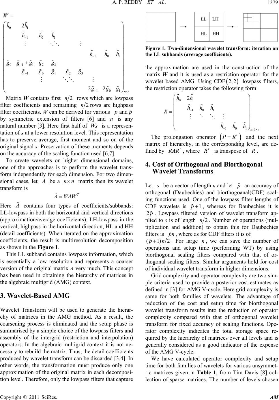
To create wavelets on higher dimensional domains,
one of the approaches is to perform the wavelet trans-
form independently for each dimension. For two dimen-
sional cases, let
A
be a nn matrix then its wavelet
transform is 

T
A
WAW
Here
A
 contains four types of coefficients/subbands:
LL-lowpass in both the horizontal and vertical directions
(approximation/average coefficients), LH-lowpass in the
vertical, highpass in the horizontal direction, HL and HH
(detail coefficients). When iterated on the approximation
coefficients, the result is multiresolution decomposition
as shown in the Figure 1.
This LL subband contains lowpass information, which
is essentially a low resolution and represents a coarser
ver sion o f the o rigin al matr ix A very much. This concept
has been used in obtaining the hierarchy of matrices in
the algebraic multigrid (AMG) context.
3. Wavelet-Based AMG
Wavelet Transform will be used to generate the hierar-
chy of matrices in the AMG method. As a result, the
coarsening process is eliminated and the setup phase is
summarised by a simple choice of the lowpass filters and
assembly of the intergrid (restriction and interpolation)
operators. In the algebraic multigrid context it is not ne-
cessary to rebuild the matrix. Thus, the detail coefficients
produced by wavelet transform can be discarded [3,4]. In
other words, the transformation must produce only one
approximation of the original matrix in each decomposi-
tion level. Th erefore, on ly the lowp ass filters that cap ture
Figure 1. Two-dimensional wavelet transform: iteration on
the LL subbands (average coefficients).
the approximation are used in the construction of the
matrix W and it is used as a restriction operator for the
wavelet based AMG. Using CDF lowpass filters,
the restriction operator takes the following form:

2,2

01
101
101
/2
2
nn
hh
hhh
R
hhh














The prolongation operator and the next
matrix of hierarchy, in the corresponding level, are de-
fined by , where is transpose of .

T
PR

T
RAR T R R
4. Cost of Orthogonal and Biorthogonal
Wavelet Transforms
Let
s
be a vector of length n and let an accuracy of
orthogonal (Daubechies) and biorthogoanal(CDF) scal-
ing functions used. One of the lowpass filter lengths of
CDF wavelets is
p

1p

, whereas for Daubechies it is
. Lowpass filtered version of wavelet transform ap-
plied to s is of length
2p

2n. Number of operations (mul-
tiplication and addition) to obtain this for Daubechies
filters is , where as for CDF filters it is of
pn

(1p)2n

. For large , we can save the number of
operations and setup time (performing WT) by using
biorthogonal scaling filters compared with that of or-
thogonal scaling filters. Similar arguments hold for cost
of individual wavelet transform in higher dimensions.
n
Grid complexity and operator complexity are two sim-
ple criteria used to provide a posterior cost estimates as
defined in [3] for AMG V-cycle. Here grid complexity is
same for both families of wavelets. The advantage of
reduction of the cost and setup time for biorthogonal
wavelet transform results into the reduction of operator
complexity compared with that of orthogonal wavelet
transform for fixed accuracy of scaling functions. Ope-
rator complexity indicates the total storage space re-
quired by the hierarchy of matrices over all levels and is
generally considered as a good indicator of the expense
of the AMG V-cycle.
We have calculated operator complexity and setup
time for both fa milies of wavelets for various un symmet-
ric matrices given in Table 1, from Tim Davis [8] col-
lection of sparse matrices. The number of levels chosen

A. P. REDDY ET AL. 1380
Table 1. Operator complexity and setup phase cputime in seconds (number in square bracket) for various matrices.
Matrix Name and size Daub-2 CDF(2,2) Daub-3 CDF(3,3)
Poisson 2D
[367 × 367] 6.65 [0.0156] 4.62 [0.0156] 10.02 [0.0312] 6.59 [0.0312]
Sherman4
[1104 × 1104] 4.23 [0.0372] 3.35 [0.0364] 6.09 [0.0374] 4.20 [0.0312]
Thermal
[3456 × 3456] 2.23 [0.0936] 1.89 [0.0728] 2.56 [0.1248] 2.26 [0.0988]
Airfoil_2D
[14214 × 14214] 6.35 [0.9100] 4.79 [0.7800] 9.00 [1.3988] 6.34 [0.9880]
Epb1
[14734 × 14734] 3.08 [0.6136] 2.53 [0.5720] 4.25 [0.8840] 3.08 [0.7124]
Epb2
[25228 × 25228] 3.25 [1.5756] 2.62 [1.3468] 4.52 [2.3192] 3.25 [1.7316]
Table 2. Convergence details: Numbers in the columns represent the required number of iterations for the convergence of the
respective method and number in square bracket represents the cputime in seconds.
Matrix Name Daub-2 CDF(2,2) Daub-3 CDF(3,3)
Poisson 2D 12
[0.2496] 13 [0.2340] 13 [0.3120] 13 [0.2704]
Sherman4 9
[0.2236] 9 [0.2288] 8 [0.2496] 9 [0.2444]
Thermal 4
[0.5148] 5 [0.6084] 5 [0.7176] 5 [0.7020]
Airfoil_2D 80
[72.9821] 78 [59.9510] 82 [103.6990] 75 [70.8433]
Epb1 129
[67.7866] 111 [52.3933] 124 [87.9266] 92 [52.6299]
Epb2 49
[35.3999] 45 [28.2733] 48 [46.7166] 41 [31.3933]
6. Conclusions
is such that in the coarsest level the dimension is less
than 100, using the expression levels = ceil(log2(n/15)),
where n is the dimension of the matrix and ceil(x):
rounds x to the nearest integer towards minus infinity.
For a given accuracy of scaling functions, precondition-
ers designed here have shorter cputime and lower opera-
tor complexity leading to reduction of cumulative trun-
cation errors, storage space and improvement of overall
accuracy, which are illustrated with examples given in
Tables 1 and 2. These two con cepts play a cruc ial role in
scientific computing. The preconditioners developed
here can also be used for other Krylov subspace iterative
methods.
5. Numerical Experiments
To test the efficiency of biorthogonal wavelet based
AMG preconditioners and compare with orthogonal wave-
let based AMG preconditioners, we have considered the
examples given in Table 1. The right hand side of linear
system was computed from the solution vector
x
of all
ones (except for Sherman4 matrix). The initial guess is
always x0 = 0 and stopping criteria is relative residual is
less than or equal to and the Krylov subspace me-
thod adapted is GMRES (20) [1]. Besides these Gauss-
Seidel is used as smoother with number of iterations
taken as two. These algorithms are implemented using
Matlab-7.5 and Mathematica-7 over machine with Intel
Core 2 Duo processor of 1.5 GHz, 667 MHz FSB and 3
GB RAM corresponding results are shown in Table 2.
6
10
7. Acknowledgements
This research work is supported by DST (SR/S4/MS:
281/05), N. M. Bujurke acknowledges the financial sup-
port of INSA, New Del hi .
8. References
[1] Y. Saad, “Iterative Methods for Sparse Linear Systems,”
SIAM, Philadelphia, 2003.
doi:10.1137/1.9780898718003
Computed results given in Tables 1 and 2 show that
the biorthogonal wavelet based preconditioners devel-
oped here, give reduction in operator complexity and
require lesser/same number of iterations or cputime. This
enables in obtaining solution of required accuracy.
[2] B. V. R. Kumar and M. Mehra, “Wavelet Based Precon-
ditioners for Sparse Linear systems,” Applied Mathemat-
ics and Computation, Vol. 171, No. 1, 2005, pp. 203-224.

A. P. REDDY ET AL.1381
doi:10.1016/j.amc.2005.01.060
[3] F. H. Pereira, S. L. L. Verardi and S. I. Nabe ta, “A Wa ve-
let-Based Algebraic Multigrid Preconditioner for Sparse
Linear Systems,” Applied Mathematics and Computation,
Vol. 182, No. 2, 2006, pp. 1098-1107.
doi:10.1016/j.amc.2006.04.057
[4] V. M. Garcia, L. Acevedo and A. M. Vidal, “Variants of
Algebraic Wavelet Based Multigrid Methods: Applica-
tions to Shifted Linear Systems,” Applied Mathematics
and Computation, Vol. 202, No. 1, 2008, pp. 287-299.
doi:10.1016/j.amc.2008.02.015
[5] A. Cohen, I. Daubechies and J. C. Feauveau, “Bior-
thogonal Bases of Compactly Supported Wavelets,” Com-
munications on Pure and Applied Mathematics, Vol. 45,
No. 5, 1992, pp. 485-560.
doi:10.1002/cpa.3160450502
[6] F. Keinert, “Wavelets and Multiwavelets,” Champan &
Hall/CRC Press, Boca Raton, 2004.
[7] W. Sweldens and P. Schroder, “Building Your Own
Wavelets at Home,” In Wavelets in Computer Graphics,
ACM SIGGRAPH course notes, 1996, pp. 15-87.
[8] T. Davis, University of Florida Sparse Matrix Collection,
NA Digest, 1997.
http://www.cise.ufl.edu/research/sparse/matrices/