Journal of Intelligent Learning Systems and Applications, 2011, 3, 249-256
doi:10.4236/jilsa.2011.34028 Published Online November 2011 (http://www.SciRP.org/journal/jilsa)
249
A New Dynamic Self-Organizing Method for
Mobile Robot Environment Mapping
Xiaogang Ruan, Yuanyuan Gao, Hongjun Song, Jing Chen
Institute of Artificial Intelligence and Robots, Beijing University of Technology, Beijing, China.
Received June 19th, 2011; revised July 19th, 2011; accepted August 1st, 2011.
ABSTRACT
To solve the mapping problem for the mobile robots in the unknown environment, a dynamic growing self-organizing
map with growing-threshold tuning automatically algorithm (DGSOMGT) based on Self-org anizing Map is proposed. It
introduces a value of spread factor to describe the changing process of the growing threshold dynamically. The method
realizes the network structure growing by training through mobile robot movement constantly in the unknown environ-
ment. The proposed algorithm is based on self-o rganizing map and can adju st the growing-thresho ld value by the num-
ber of network neurons increasing. It avoids tuning the parameters repeatedly by human. The experimental results show
that the proposed method detects the comp lex environment qu ickly, effectively and correctly. The robot can realize en-
vironment mapping automatically. Compared with the other methods the proposed mapping strategy has better topo-
logical properties and time property.
Keywords: Mobile Robot, Environment Mapping, Growing-Thresh old Tuning, Sel f-Organizing
1. Introduction
The ultimate goal of mobile robotics research is to endow
the robots with high autonomous ability, of which navi-
gation in an unknown environment is achieved by using
on-line sensory information. First a correct environment
model is usually needed and the robot can update the
model by using sensory information. It is a key problem
that the robot is able to map the environment automati-
cally. A significant amount of research effort has been
devoted to this area in the past decades such as probabil-
ity grid [1], geometry algorithm [2], topology informa-
tion [3] and the 3D information methods [4]. The defi-
ciency of geometry algorithm is that feature extraction is
very difficult, especially in the complex environment. On
the other hand, the topological method has the higher
efficiency and smaller memory space. It is suitable for
the large-scale work space. By this approach, main con-
cern lays in finding the most effective way to map the
environment while simultaneously localizing the robot’s
position relative to the map. If just th e accur ate map were
acquired, then the shortest path would be easily obtain-
able from the occupancy grid map [5]. However, to ac-
quire such map in an unknown environment is not easy.
The robot moves in the unfamiliar and non-stationary
environment and doesn’t know any prior knowledge.
Network growth is an important feature to adapt to
non-stationary environments. Many conventional cluste-
ring algorithms such as k-means demand that a user pre-
determine how many clusters are to be generated. For a
topology learning problem, a user of many conventional
methods like Kohonen Feature Map [6] must decide the
number of nodes in advance.
Nehmzow and Smithers have used Kohonen’s Self-
organizing Maps (SOMs) to endow their robots with map
building abilities [7]. Their approach to mapping is bas-
ed on the correlations that exist between the sensor data
representing a fixed environment and the motor respon-
ses of the robot. Najand et al. have been working along
the same line using TPM (Topology Preserving Mapping)
networks. They studied problems associated with pa-
rameters which affect the learning process [8]. V. More-
llas, et al. proposed an approach which puts emphasizes
the dynamic interaction between th e mobile ro bot an d th e
environment and attempts to bridge the gap between Ar-
tificial Intelligence (AI) techniques and behavior-based
methodologies [9]. A major problem with this solution is
that the set of vertices corresponding to the objects of the
environment must be known a priori, which in gener- al,
is a difficult and computati onally tim e consumi ng task.
Incremental learning addresses the ability of repeat-
edly training a network using new data without destroy-

A New Dynamic Self-Organizing Method for Mobile Robot Environment Mapping
250
ing the old prototype patterns. Incremental learning is
useful in many applications. For example, if we intend to
bridge the gap between the learning capabilities of hu-
mans and machines, we must consider which circumsta-
nces allow a sequential acquisition of knowledge. The
fundamental issue for incremental learn ing is how a lear-
ning system can adapt to new information without cor-
rupting or forgetting previously learned information [10].
In recent years, many scholars have also applied some
methods of incremental learning to the robot environ-
ment map. Oishi, T. et al. designs the architecture of a
self creating and or ganizing neural network for workspa-
ce recognition and navigation of an autonomous mobile
robot. Methods of path planning and navigation based on
a topological map created by learning are also proposed.
The proposed architecture was tested by simulation of an
autonomous mobile robot with eight sonar sensors, and it
was demonstrated that the architecture is useful for the
purpose [11]. Gyu-jong Choi used the topological form
to build the environment map [12]. Y. Zhuang et al. had
maked use of the geometry-topoloty hybrid approach
[13]. A. Kawewong et al. used an approach based on the
associative memory using Self-Organizing Incremental
Neural Networks (SOINN) because it is suitable to noisy
environment and is easily implemented [14]. Ruan et al.
presented an algorithm of Dynamic Growing Self-orga-
nizing (DGSOM) using in building environment [15]. It
is simple and effective but the static value of Growing
Threshold (GT) is used which can not realize mapping
quickly.
However, it is not easy to define appropriate search
and memory space. To solve this problem, a dynamic
growing self-organizing map with growing-threshold au-
tonomic tuning algorithm (DGSOMGT) based on Self-
organizing Map is proposed and it is used in environment
mapping. The spread factor (SF) is introduced to describe
the degree of TPM. The value of GT changes with the
value of SF. If SF is smaller, GT is bigger and it can re-
alize the lower clustering. Or else, it can realize the hi-
gher clustering. The propo sed algorithm is based on self-
organizing map and can adjust the growing-threshold va-
lue by the number of network neurons increasing. It av-
oids tuning the parameters repeatedly by human. The ex-
perimental results show that the proposed method detects
the complex environment effectively and correctly and
the robot can realize environment mapping automatically.
Compared with the SOM method the proposed mapping
strategy has better topological properties and time.
2. SOM Algorithm Introduction
A new idea is presented by the appearance of Self-orga-
nizing Map. The Kohonen featur e map [6] allows projec-
tion onto non-linear, discretely sampled subspaces of a
dimensionality. But it requires predetermination of the
network structure and network size. The combination of
“competitive Hebbian learning” (CHL) and “neural gas”
(NG) [16] also requires a prior decision about the net-
work size. Therefore, the Growing Cell Structur e [17], Self-
Creating and Organizing Neural Networks [18] and Grow-
ing Self-Organizing Map [19] were presented to solve the
problem in the information processing field such as im-
age processing, pattern recognition and data compression.
Shen and Hasegawa proposed an incremental learning
method called the self-organizing incremental neural net-
work (SOINN) [20] to realize the unsupervised incre-
mental learning task. In fact, SOINN is useful to process
online non-stationary data, report a suitable number of cl-
asses, and represent the topological structure of input
probability density. An enhanced self-organizing incre-
mental neural network (ESOINN) [10] is proposed to ac-
complish online unsupervised learning tasks. It improves
the self-organizing incremental neural network (SOINN).
The above methods are all based on the algorithm of
SOM. Here we introduce the process of SOM firstly.
An n-rank SOM of n-dimensional input space can be
determined exclusively by the feed forward synaptic con-
nection. It has two layers o f the input layer and competi-
tive layers. Competition, cooperation and synaptic adap-
tation constitute are the three basic aspects of SOM ope-
rational mechanism.
1) SOM Competition mechanism
SOM competition mechanism is:



min T
j
ix
ox xw (1)
where x is the input of stimulus.

ix
vis the connection
weight of the neuron number of j.


ix
ox is the output
of winning unit. Neuron ()ix v will become the winning
unit which is stimulated by x. The winning SOM neuron

ix
v is the excited centre of SOM sensory field which is
stimulate by x.
2) SOM Cooperation Mechanism
Winning SOM neurons sets up a topological neigh-
borhood with taking itself as the center. Like in biologi-
cal nervous system, the winning neuron stimulates neigh-
borhood neurons to excite together with a distribution si-
milar to Mexican Hat Function. Neighborhood function
can be a square wave function or a Gaussian function.
The most commonly use are Gaussian functions:

2
()
() 2
exp1,2, ,
2
ixj
ixj
djN



 



 (2)
where

is the effective radius of Gaussian neighbor-
hood,

is lateral distance, that is, Euclidean distance
between neuron
j
vand the winning neuron .
3) SOM Synaptic Adaptation Mechanism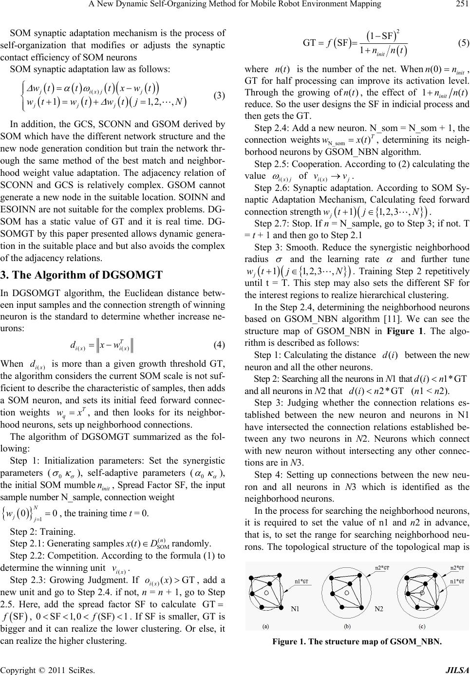

A New Dynamic Self-Organizing Method for Mobile Robot Environment Mapping
251
SOM synaptic adaptation mechanism is the process of
self-organization that modifies or adjusts the synaptic
contact efficiency of SOM neurons
SOM synaptic adaptation law as follows:
 
 


()
11,2,,
jixjj
jjj
wt ttxwt
wtwtwt jN




 

 (3)
In addition, the GCS, SCONN and GSOM derived by
SOM which have the different network structure and the
new node generation condition but train the network thr-
ough the same method of the best match and neighbor-
hood weight value adaptation. The adjacency relation of
SCONN and GCS is relatively complex. GSOM cannot
generate a new node in the suitable location. SOINN and
ESOINN are not suitable fo r the complex problems. DG-
SOM has a static value of GT and it is real time. DG-
SOMGT by this paper presented allows dynamic genera-
tion in the suitable place and but also avoids the complex
of the adjacency relations.
3. The Algorithm of DGSOMGT
In DGSOMGT algorithm, the Euclidean distance betw-
een input samples and the connectio n streng th of winn ing
neuron is the standard to determine whether increase ne-
urons:
() ()
T
ix ix
dxw (4)
When ()ix d is more than a given growth threshold GT,
the algorithm considers the current SOM scale is not suf-
ficient to describe the ch aracteristic of samples, then adds
a SOM neuron, and sets its initial feed forward connec-
tion weights T
q
wx, and then looks for its neighbor-
hood neurons , set s up nei g hb or h oo d co nnections.
The algorithm of DGSOMGT summarized as the fol-
lowing:
Step 1: Initialization parameters: Set the synergistic
parameters (0


 ), self-adaptive parameters (0



),
the initial SOM mumbleinit n, Spread Factor SF, the input
sample number N_sample, connection weight
 
1
00
N
jj
w, the training tim e t = 0.
Step 2: Training.
Step 2.1: Generating samples()
SOM
() n xt Drandomly.
Step 2.2: Competition. According to the formula (1) to
determine the winning unit ()ix v.
Step 2.3: Growing Judgment. If () () GT
ix
ox, add a
new unit and go to Step 2.4. if not, n = n + 1, go to Step
2.5. Here, add the spread factor SF to calculate GT


SF ,f0SF1,0 (SF)1f . If SF is smaller, GT is
bigger and it can realize the lower clustering. Or else, it
can realize the higher clustering.
 

2
1SF
GTSF 1init fnnt


 (5)
where ()nt is the number of the net. When(0) init nn

,
GT for half processing can improve its activation level.
Through the growing of()nt , the effect of 1()
init
nnt

reduce. So the user designs the SF in indicial process and
then gets the GT.
Step 2.4: Add a new neuron. N_som = N_som + 1, the
connection weightsN_som ()
T
wxt, determining its neigh-
borhood neurons by GSOM_NBN algorithm.
Step 2.5: Cooperation. According to (2) calculating the
value ()ixj

of ()ix j vv.
Step 2.6: Synaptic adaptation. According to SOM Sy-
naptic Adaptation Mechanism, Calculating feed forward
connection strength

  
11,2,3,
j
wt jN .
Step 2.7: Stop. If n = N_sample, go to Step 3; if not. T
= t + 1 and then go to Step 2.1
Step 3: Smooth. Reduce the synergistic neighborhood
radius

and the learning rate

and further tune






11,2,3,
j
wt jN . Training Step 2 repetitively
until t = T. This step may also sets the different SF for
the interest regions to realize hierarchical clustering.
In the Step 2.4, determining the neighborhood neurons
based on GSOM_NBN algorithm [11]. We can see the
structure map of GSOM_NBN in Figure 1. The algo-
rithm is described as follows:
Step 1: Calculating the distance ()di between the new
neuron and all the other neurons.
Step 2: Searching all the neurons in N1 that() 1*GTdi n

and all neurons in N2 that ()2*GTdi n (n1 < n2).
Step 3: Judging whether the connection relations es-
tablished between the new neuron and neurons in N1
have intersected the connection relations established be-
tween any two neurons in N2. Neurons which connect
with new neuron without intersecting any other connec-
tions are in N3.
Step 4: Setting up connections between the new neu-
ron and all neurons in N3 which is identified as the
neighborhood neurons.
In the process for searching the neighborhood neurons,
it is required to set the value of n1 and n2 in advance,
that is, to set the range for searching neighborhood neu-
rons. The topological structure of the topological map is
Figure 1. The structure map of GSOM_NBN.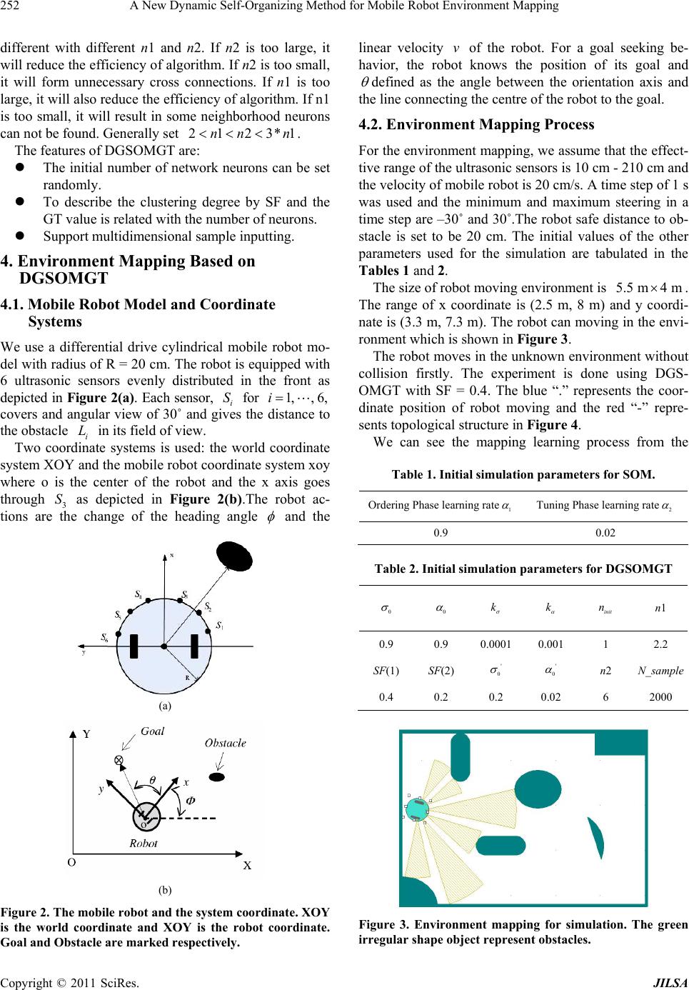

A New Dynamic Self-Organizing Method for Mobile Robot Environment Mapping
252
different with different n1 and n2. If n2 is too large, it
will reduce the efficiency of alg orithm. If n2 is too small,
it will form unnecessary cross connections. If n1 is too
large, it will also reduce the efficiency of algorithm. If n1
is too small, it will result in some neighborhood neurons
can not be found. Generally set 2123*1nn n .
The features of DGSOMGT are:
 The initial number of network neurons can be set
randomly.
 To describe the clustering degree by SF and the
GT value is related with the number of neurons.
 Support multidimensional sample inputting.
4. Environment Mapping Based on
DGSOMGT
4.1. Mobile Robot Model and Coordinate
Systems
We use a differential drive cylindrical mobile robot mo-
del with radius of R = 20 cm. The robot is equipped with
6 ultrasonic sensors evenly distributed in the front as
depicted in Figure 2(a). Each sensor, i
S for 1,, 6,i


covers and angular view of 30˚ and gives the distance to
the obstacle i L in its field of view.
Two coordinate systems is used: the world coordinate
system XOY and the mobile robot coordinate system xoy
where o is the center of the robot and the x axis goes
through 3 S as depicted in Figure 2(b).The robot ac-
tions are the change of the heading angle

and the
(a)
(b)
Figure 2. The mobile robot and the system coordinate. XOY
is the world coordinate and XOY is the robot coordinate.
Goal and Obstacle are marked respectively.
linear velocity v of the robot. For a goal seeking be-
havior, the robot knows the position of its goal and

defined as the angle between the orientation axis and
the line connecting the centre of the robot to the go al.
4.2. Environment Mapping Process
For the environment mapping, we assume that the effect-
tive range of the ultrasonic sensor s is 10 cm - 210 cm and
the velocity of mobile robot is 20 cm/s. A time step of 1 s
was used and the minimum and maximum steering in a
time step are –30˚ and 30˚.The robot safe distance to ob-
stacle is set to be 20 cm. The initial values of the other
parameters used for the simulation are tabulated in the
Tables 1 and 2.
The size of robot moving environment is 5.5 m4 m

.
The range of x coordinate is (2.5 m, 8 m) and y coordi-
nate is (3.3 m, 7.3 m). The robot can moving in the envi-
ronment which is shown in Figure 3.
The robot moves in the unkno wn environment without
collision firstly. The experiment is done using DGS-
OMGT with SF = 0.4. The blue “.” represents the coor-
dinate position of robot moving and the red “-” repre-
sents topological structure in Figure 4.
We can see the mapping learning process from the
Table 1. Initial simulation parameters for SOM.
Ordering Phase learning rate1

Tuning Phase learning rate2

0.9 0.02
Table 2. Initial simulation parameters for DGSOMGT
0

0

k

k

init n n1
0.9 0.9 0.0001 0.001 1 2.2
SF(1) SF(2) '
0

'
0

n2 N_sample
0.4 0.2 0.2 0.02 6 2000
Figure 3. Environment mapping for simulation. The green
irregular shape object represent obstacles.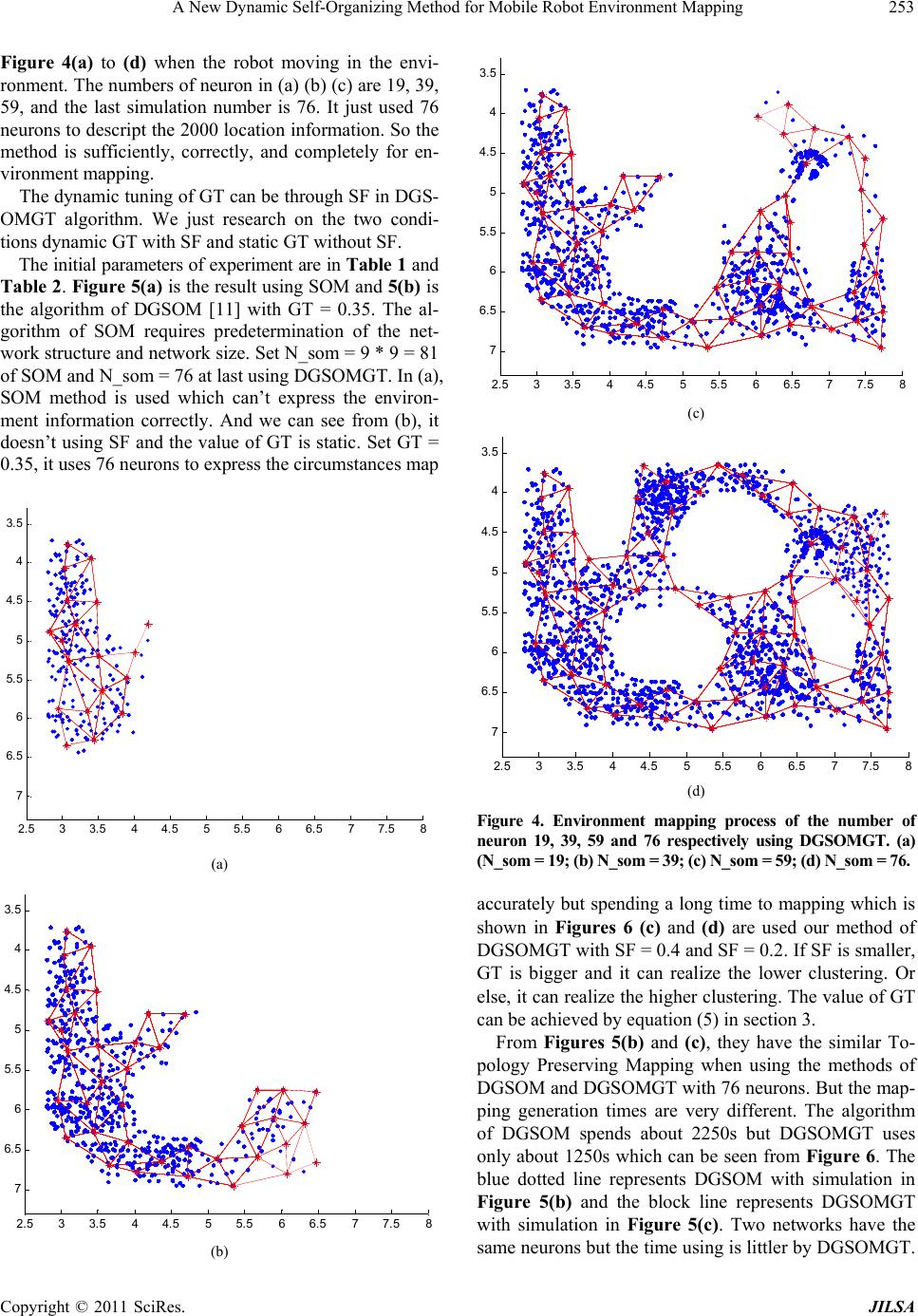

A New Dynamic Self-Organizing Method for Mobile Robot Environment Mapping
253
Figure 4(a) to (d) when the robot moving in the envi-
ronment. The numbers of neuron in (a) (b) (c) are 19, 39,
59, and the last simulation number is 76. It just used 76
neurons to descript the 2000 location information. So the
method is sufficiently, correctly, and completely for en-
vironment mapping.
The dynamic tuning of GT can be through SF in DGS-
OMGT algorithm. We just research on the two condi-
tions dynamic GT with SF and static GT without SF.
The initial para meters of experiment are in Table 1 and
Table 2. Figure 5( a) is the result using SOM and 5(b) is
the algorithm of DGSOM [11] with GT = 0.35. The al-
gorithm of SOM requires predetermination of the net-
work structure and network size. Set N_som = 9 * 9 = 81
of SOM and N_som = 76 at last using DGSOMGT. In (a),
SOM method is used which can’t express the environ-
ment information correctly. And we can see from (b), it
doesn’t using SF and the value of GT is static. Set GT =
0.35, it uses 76 neurons to express the circumstances map
2.5 33.544.5 55.5 66.5 77.5 8
3. 5
4
4. 5
5
5. 5
6
6. 5
7
(a)
2.5 33.5 44.5 55.5 66.5 77.5 8
3.5
4
4.5
5
5.5
6
6.5
7
(b)
2.5 33.5 44.5 55.5 66.5 77.5 8
3. 5
4
4. 5
5
5. 5
6
6. 5
7
(c)
2.5 33.5 44.5 55.5 66.5 77.5 8
3.5
4
4.5
5
5.5
6
6.5
7
(d)
Figure 4. Environment mapping process of the number of
neuron 19, 39, 59 and 76 respectively using DGSOMGT. (a)
(N_som = 19; (b) N_som = 39; (c) N_som = 59; (d) N_som = 76.
accurately but spending a long time to mapping which is
shown in Figures 6 (c) and (d) are used our method of
DGSOMGT with SF = 0.4 and SF = 0.2. If SF is smaller,
GT is bigger and it can realize the lower clustering. Or
else, it can realize the higher clustering. The value of GT
can be achieved by equation (5) in section 3.
From Figures 5(b) and (c), they have the similar To-
pology Preserving Mapping when using the methods of
DGSOM and DGSOMGT with 76 neurons. But the map-
ping generation times are very different. The algorithm
of DGSOM spends about 2250s but DGSOMGT uses
only about 1250s which can be seen from Figure 6. The
blue dotted line represents DGSOM with simulation in
Figure 5(b) and the block line represents DGSOMGT
with simulation in Figure 5(c). Two networks have the
same neurons but the time using is littler by DGSOMGT.

A New Dynamic Self-Organizing Method for Mobile Robot Environment Mapping
254
It is because that the value of GT is dynamic and it has a
smaller value in the early mapping when using the algori-
thm of DGSOMGT. The Topology Preserving Mapping can
grow more quickly than using the algorithm of DGSOM.
In Figures 5(c) and (d), the method of DGSOMGT is
used with differ ent SF. From Section 3 we know that the
value of SF is bigger and the Topology Preserving Map-
ping is more detailed, but the time spending is growing
accordingly.
In the real time Topology Preserving Mapping, time
consumption is a very important performance to identify
the algorithm practicality.
Figure 6 shows the three growing curves of neuron
number with the time consumption using the algorithm
of DGSOM and DGSOMGT with SF = 0.4 and SF = 0.2.
We can see that two networks have the same neurons but
the time consumption is different using DGSOM with
GT = 0.35 and DGSOMGT with SF = 0.4 which the
value of GT is changing from 0.18 to 0.35. The time con-
sumption of DGSOM is longest which is about 2250s,
2.5 33.5 44.5 55.5 66.5 77.5 8
3.5
4
4.5
5
5.5
6
6.5
7
W(i ,1)
W(i,2)
Weight Vectors
(a)
2.5 33.5 44.5 55.5 66.5 77.5 8
3.5
4
4.5
5
5.5
6
6.5
7
(b)
3 4 5 6 7 8
3.5
4
4.5
5
5.5
6
6.5
7
(c)
2.5 33.5 44.5 55.5 66.5 77.5 8
3.5
4
4.5
5
5.5
6
6.5
7
(d)
Figure 5. The experiments of environment mapping are
realized by SOM, DGSOM and DGSOMGT respectively.
The X-axis is the horizontal ordinate of 2D environment,
and the Y-axis is the vertical coordinates. The simulation
experiments using DGSOM with static GT = 0.25, and
DGSOMGT with SF = 0.4 and with SF = 0.2.
and DGSOMGT with SF = 0.4 which is about 1250s.
The time is reduced by about 1000s wh en introducing SF.
The red dotted line represents the result of DGSOMGT
with SF = 0.2. It has the shortest time but not correct des-
cription when the value GT changes from 0.33 to 0.58.
The values of GT are too big for mapping when SF is
equal to 0.2. At last, we find a more suited value of SF to
building the environment mapping which SF is equal to
0.4 consideration of TPM and time consumption.
Figure 7 shows the change value of GT with the robot
moving in the environment when SF is equal to 0.4 and
0.2. When the value of SF is bigger, the GT is smaller
and it can describe the environment accurately but time
consuming. If the value of SF is too smaller, the Topol-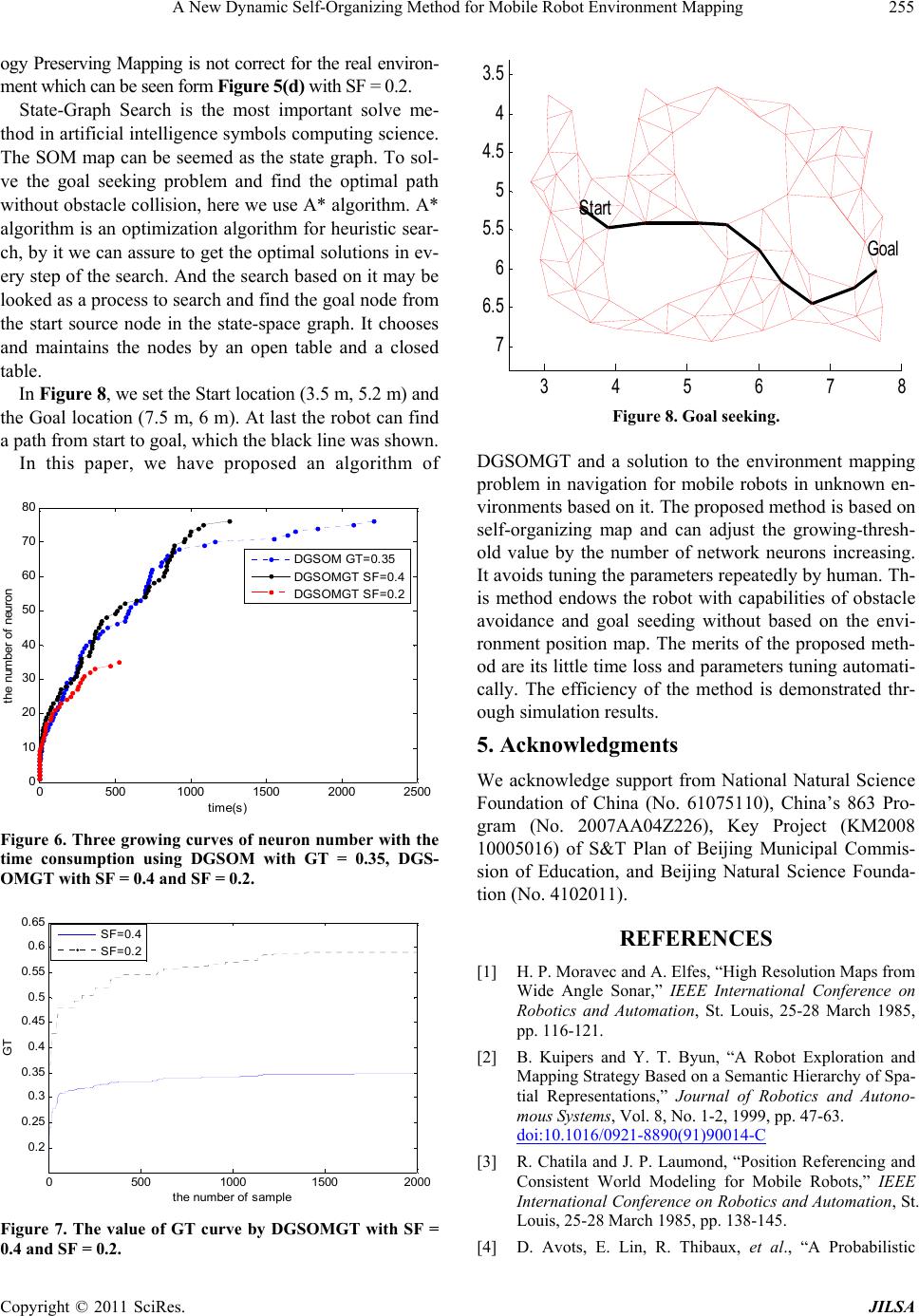

A New Dynamic Self-Organizing Method for Mobile Robot Environment Mapping
255
ogy Preserv ing Mapping is not correc t for the real environ-
ment which can be seen form Figure 5(d) with SF = 0.2.
State-Graph Search is the most important solve me-
thod in artificial intelligence symbols co mputing science.
The SOM map can be seemed as the state graph. To sol-
ve the goal seeking problem and find the optimal path
without obstacle collision, here we use A* algorithm. A*
algorithm is an optimization algorith m for heuristic sear-
ch, by it we can assure to get the optimal solutions in ev-
ery step of the search. And the search based on it may be
looked as a process to search and find the goal node from
the start source node in the state-space graph. It chooses
and maintains the nodes by an open table and a closed
table.
In Figure 8, we set the Start location (3.5 m, 5.2 m) and
the Goal location (7.5 m, 6 m). At last the robot can find
a path from start to goal, which the black line was shown.
In this paper, we have proposed an algorithm of
05001000 1500 2000 2500
0
10
20
30
40
50
60
70
80
time(s)
the number of neuron
DGSO M GT =0.35
DGSOMGT SF=0.4
DGSOMGT SF=0.2
Figure 6. Three growing curves of neuron number with the
time consumption using DGSOM with GT = 0.35, DGS-
OMGT with SF = 0.4 and SF = 0.2.
05001000 15002000
0. 2
0. 25
0. 3
0. 35
0. 4
0. 45
0. 5
0. 55
0. 6
0. 65
t he num ber of sampl e
GT
SF=0.4
SF=0.2
Figure 7. The value of GT curve by DGSOMGT with SF =
0.4 and SF = 0.2.
3 4 5 6 7 8
3.5
4
4.5
5
5.5
6
6.5
7
Goal
Start
Figure 8. Goal seeking.
DGSOMGT and a solution to the environment mapping
problem in navigation for mobile robots in unknown en-
vironments based on it. The proposed method is based on
self-organizing map and can adjust the growing-thresh-
old value by the number of network neurons increasing.
It avoids tuning the parameters repeatedly by human. Th-
is method endows the robot with capabilities of obstacle
avoidance and goal seeding without based on the envi-
ronment position map. The merits of the proposed meth-
od are its little ti me loss and parameters tuning automati-
cally. The efficiency of the method is demonstrated thr-
ough simulation results.
5. Acknowledgments
We acknowledge support from National Natural Science
Foundation of China (No. 61075110), China’s 863 Pro-
gram (No. 2007AA04Z226), Key Project (KM2008
10005016) of S&T Plan of Beijing Municipal Commis-
sion of Education, and Beijing Natural Science Founda-
tion (No. 4102011).
REFERENCES
[1] H. P. Moravec and A. Elfes, “High Resolution Maps from
Wide Angle Sonar,” IEEE International Conference on
Robotics and Automation, St. Louis, 25-28 March 1985,
pp. 116-121.
[2] B. Kuipers and Y. T. Byun, “A Robot Exploration and
Mapping Strategy Based on a Semantic Hierarchy of Spa-
tial Representations,” Journal of Robotics and Autono-
mous Systems, Vol. 8, No. 1-2, 1999, pp. 47-63.
doi:10.1016/0921-8890(91)90014-C
[3] R. Chatila and J. P. Laumond, “Position Referencing and
Consistent World Modeling for Mobile Robots,” IEEE
International Conference on Robotics and Automation, St.
Louis, 25-28 March 1985, pp. 138-145.
[4] D. Avots, E. Lin, R. Thibaux, et al., “A Probabilistic

A New Dynamic Self-Organizing Method for Mobile Robot Environment Mapping
256
Technique for Simultaneous Localization and Door State
Estimation with Mobile Robots in Dynamic Environ-
ments,” Proceedings of IEEE/RSJ International confer-
ence on Intelligent Robots and System, Lausanne, 30
September-5 October 2002, pp. 521-526.
[5] B. Kuipers, J. Modayil, P. Beeson, M. Macmahon and F.
Savelli, “Local Metrical and Global Topological Maps in
the Hybrid Spatial Semantic Hierarchy,” Proceedings of
International conference on Robotics and Automation,
New Orleans, 26 April-1 May 2004, pp. 4845-4851.
[6] T. Kohonen, “Self-Organized Formation of Topologically
Correct Feature Maps,” Biological Cybernetics, Vol. 43,
No. 1, 1982, pp. 59-69. doi:10.1007/BF00337288
[7] U. Nehmzow and T. Smithers, “Mapbuilding Using Self-
Organizing Networks in Really Useful Robots,” From
Animals to Animats: Proceedings of the First Interna-
tional Conference on Simulation of Adaptive Behavior,
Paris, 24-28 September 1991, pp. 152-159.
[8] S. Najand, Z. Lo and B. Bavarian, “Application of Self-
Organizing Neural Networks for Mobile Robot Environ-
ment Learning,” Neural Network in Robotics, Kluwer
Academic Publishers, Vol. 202, No. 1, 1993, pp. 85-96.
[9] V. Morellas, J. Minners and M. Donath, “Implementation
of Real Time Spatial Mapping in Robotic Systems throu-
gh Self-Organizing Neural Networks,” Proceedings of
1995 IEEE/RSJ International Conference on Intelligent
Robots and Systems. Human Robot Interaction and Co-
operative Robots, Vol. 1, Pittsburgh, 5-9 August 1995, pp.
277-284.
[10] F. Shen, O. Ha segawa and H. Osamu, “An Enhan ced Self-
Organizing Incremental Neural Network for Online Un-
supervised Learning,” Neural Networks, Vol. 20, No. 8,
2007, pp. 893-903. doi:10.1016/j.neunet.2007.07.008
[11] T. Oishi, K. Furuta and S. Kondo, “Workspace Recogni-
tion and Navigation of Autonomous Mobile Robot Using
Self-Creating and Organizing Neural Network,” Transac-
tion of the Society of Instrument and Dontrol Engineers,
Vol. 33, No. 3, 1997, pp. 203-208.
[12] G. J. Choi and D. S. Ahn, “Map Building and Localiza-
tion on Autonomous Mobile Robot Using Graph and Fu-
zzy Inference System,” IEEE International Joint Confer-
ence on Neural Networks, Budapest, 25-29 July 2004, pp.
2419-2424.
[13] Y. Zhuang, X. D. Xu and W. Wang, “Mobile Robot Geo-
metric-Topological Map Building and Self-Localization,”
Control and Decision, Vol. 20, No. 7, 2005, pp. 815-818.
[14] A. Kawewong, Y. Honda, M. Tsuboyama and O. Hasega-
wa, “Reasoning on the Self-Organizing Incremental As-
sociative Memory for Online Robot Path Planning,”
IEICE Transactions on Information and Systems, Vol.
E93-D, No. 3, 2010, pp. 569-582.
[15] X. G. Ruan and X. T. Xing, “Application of Autonomous
Mapping Algorithm on a Desktop Robot System,” Pro-
ceedings of the 5th International Conference on Natural
Computation, Tianjin, 14-16 August 2009, pp. 448-453.
doi:10.1109/ICNC.2009.156
[16] T. M. Martinetz, S. G.Berkovich and K. J. Schulten, “Neu-
ral-Gas Network for Vector Quantization and Its Applica-
tion to Ime-Series Prediction,” IEEE Transaction s on Neu-
ral Networks, Vol. 4, No. 4, 1996, pp. 558-569.
doi:10.1109/72.238311
[17] B. Fritzke, “Growing Cell Structures—A Self-Organizing
Network for Unsupervised and Supervised Learning,”
Neural Network, Vol. 7, No. 9, 1994, pp. 1411-1460.
doi:10.1016/0893-6080(94)90091-4
[18] D. Choi and S. Park, “Self-Creating and Organizing Neu-
ral Networks,” IEEE Transactions on Neural Networks,
Vol. 5, No. 4, 1994, pp. 561-575. doi:10.1109/72.298226
[19] D. Alahakoon and S. K. Halgamuge, “Dynamic Self-Orga-
nizing Maps with Controlled Growth for Knowledge Dis-
covery,” IEEE Transactions on Neural Networks, Vol. 11,
No.3, 2000, pp. 601-614. doi:10.1109/72.846732
[20] F. Shen and O. Hasegawa, “An Incremental Network for
On-Line Unsupervised Classification and Topology Lear-
ning,” Neural Networks, Vol. 19, 2006, pp. 90-106.
doi:10.1016/j.neunet.2005.04.006