Recurrent Support and Relevance Vector Machines Based Model with Application to Forecasting Volatility of Financial Returns

doi:10.4236/jilsa.2011.34026

Paper Menu >>

Journal Menu >>

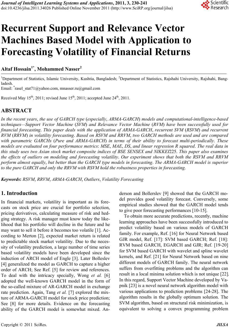
Journal of Intelligent Learning Systems and Applications, 2011, 3, 230-241

doi:10.4236/jilsa.2011.34026 Published Online November 2011 (http://www.SciRP.org/journal/jilsa)

Recurrent Support and Relevance Vector

Machines Based Model with Application to

Forecasting Volatility of Financial Returns

Altaf Hossain1*, Mohammed Nasser2

1Department of Statistics, Islamic University, Kushtia, Bangladesh; 2Department of Statistics, Rajshahi University, Rajshahi, Bang-

ladesh.

Email: *rasel_stat71@yahoo.com, mnasser.ru@gmail.com

Received May 15th, 2011; revised June 15th, 2011; accepted June 24th, 2011.

ABSTRACT

In the recent years, the use of GARCH type (especially, ARMA-GARCH) models and computational-intelligence-based

techniques—Support Vector Machine (SVM) and Relevance Vector Machine (RVM) have been successfully used for

financial forecasting. This paper deals with the application of ARMA-GARCH, recurrent SVM (RSVM) and recurrent

RVM (RRVM) in volatility forecasting. Based on RSVM and RRVM, two GARCH methods are used and are compared

with parametric GARCHs (Pure and ARMA-GARCH) in terms of their ability to forecast multi-periodically. These

models are evaluated on four performance metrics: MSE, MAE, DS, and linear regression R squared. The real data in

this study uses two Asian stock market composite indices of BSE SENSEX and NIKKEI225. This paper also examines

the effects of outliers on modeling and forecasting volatility. Our experiment shows that both the RSVM and RRVM

perform almost equally, but better than the GARCH type models in forecasting. The ARMA-GARCH model is superior

to the pure GARCH and only the RRVM with RSVM hold the robustness properties in forecasting.

Keywords: RSVM, RRVM, ARMA-GARCH, Outliers, Volatility Forecasting

1. Introduction

In financial markets, volatility is important as its fore-

casts on stock price are crucial for portfolio selection,

pricing derivatives, calculating measure of risk and hed-

ging strategy. A risk manager must know today the like-

lihood that his portfolio will decline in the future and he

may want to sell it before it becomes too volatile [1]. Ac-

cording to Merton [2], expected market return is related

to predictable stock market volatility. Due to the neces-

sity of volatility prediction, a large number of time series

based volatility models have been developed since the

induction of ARCH model of Engle [3]. Later Bolleslev

[4] generalized the model as GARCH to capture a higher

order of ARCH; See Ref. [5] for review and references.

To deal with the intricacy specially, Wong et al. [6]

adopted the well-known GARCH model in the form of

the so-called mixture of AR-GARCH model in exchange

rate prediction. Again, Tang et al. [7] explored the mix-

ture of ARMA-GARCH model for stock price prediction;

See [8] for more details. Evidence on the forecasting

ability of the GARCH model is somewhat mixed. An-

derson and Bollerslev [9] showed that the GARCH mo-

del provides good volatility forecast. Conversely, some

empirical studies showed that the GARCH model tends

to give poor forecasting performances [10-15].

To obtain more accurate predictions, recently, machine

learning approaches have been successfully introduced to

predict volatility based on various models of GARCH

family. For example, Ref. [16] for Neural Network based

GJR model, Ref. [17]: SVM based GARCH; Ref. [18]:

RVM based GARCH, EGARCH and GJR; Ref. [19-20]

for SVM based GARCH with wavelet and spline wavelet

kernels, and Ref. [21] for Neural Network based on nine

different models of GARCH family. The neural network

suffers from overfitting problems and the algorithm can

result in a local minima solution which is not unique [22].

In this regard, Support Vector Machine developed by Va-

pnik [23] is a novel neural network algorithm model with

various applications to prediction problems [24-28]. The

algorithm results in the globally optimum solution. The

SVM algorithm, based on structural risk minimization, is

equivalent to solving a convex programming problem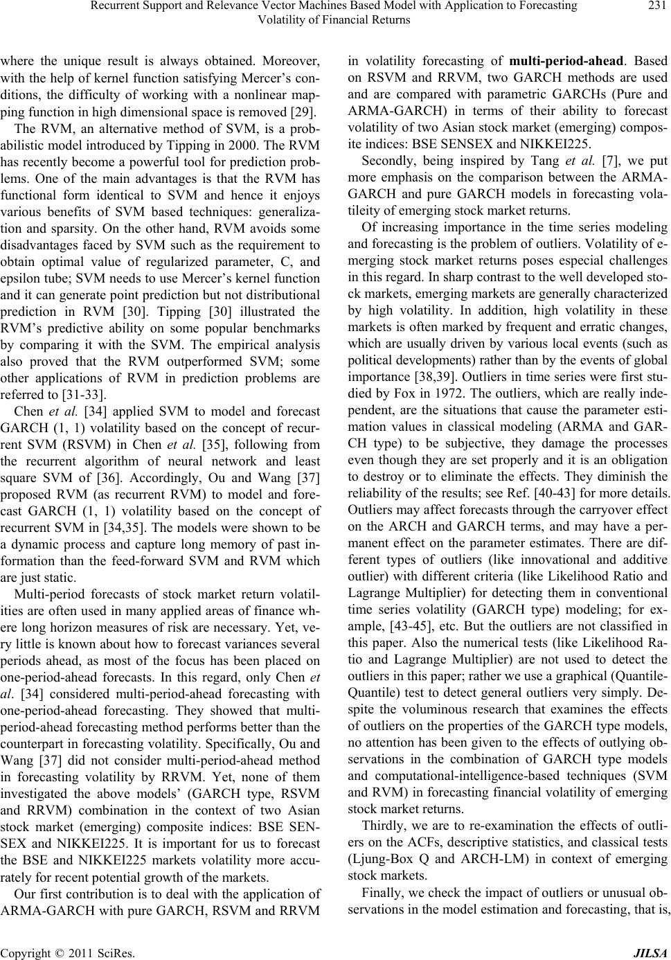

Recurrent Support and Relevance Vector Machines Based Model with Application to Forecasting 231

Volatility of Financial Returns

where the unique result is always obtained. Moreover,

with the help of kernel function satisfying Mercer’s con-

ditions, the difficulty of working with a nonlinear map-

ping function in high dimensional space is removed [29].

The RVM, an alternative method of SVM, is a prob-

abilistic model introduced by Tipping in 2000. The RVM

has recently become a powerful tool for prediction prob-

lems. One of the main advantages is that the RVM has

functional form identical to SVM and hence it enjoys

various benefits of SVM based techniques: generaliza-

tion and sparsity. On the other hand, RVM avoids some

disadvantages faced by SVM such as the requirement to

obtain optimal value of regularized parameter, C, and

epsilon tube; SVM needs to use Mercer’s kernel function

and it can generate point prediction but not distributional

prediction in RVM [30]. Tipping [30] illustrated the

RVM’s predictive ability on some popular benchmarks

by comparing it with the SVM. The empirical analysis

also proved that the RVM outperformed SVM; some

other applications of RVM in prediction problems are

referred to [31-33].

Chen et al. [34] applied SVM to model and forecast

GARCH (1, 1) volatility based on the concept of recur-

rent SVM (RSVM) in Chen et al. [35], following from

the recurrent algorithm of neural network and least

square SVM of [36]. Accordingly, Ou and Wang [37]

proposed RVM (as recurrent RVM) to model and fore-

cast GARCH (1, 1) volatility based on the concept of

recurrent SVM in [34,35]. The models were shown to be

a dynamic process and capture long memory of past in-

formation than the feed-forward SVM and RVM which

are just static.

Multi-period forecasts of stock market return volatil-

ities are often used in many applied areas of finance wh-

ere long horizon measures of risk are necessary. Yet, ve-

ry little is known about how to forecast variances several

periods ahead, as most of the focus has been placed on

one-period-ahead forecasts. In this regard, only Chen et

al. [34] considered multi-period-ahead forecasting with

one-period-ahead forecasting. They showed that multi-

period-ahead forecasting method performs better than the

counterpart in forecasting volatility. Specifically, Ou and

Wang [37] did not consider multi-period-ahead method

in forecasting volatility by RRVM. Yet, none of them

investigated the above models’ (GARCH type, RSVM

and RRVM) combination in the context of two Asian

stock market (emerging) composite indices: BSE SEN-

SEX and NIKKEI225. It is important for us to forecast

the BSE and NIKKEI225 markets volatility more accu-

rately for recent potential growth of the markets.

Our first contribution is to deal with the application of

ARMA-GARCH with pure GARCH, RSVM and RRVM

in volatility forecasting of multi-period-ahead. Based

on RSVM and RRVM, two GARCH methods are used

and are compared with parametric GARCHs (Pure and

ARMA-GARCH) in terms of their ability to forecast

volatility of two Asian stock market (emerging) compos-

ite indices: BSE SENSEX and NIKKEI225.

Secondly, being inspired by Tang et al. [7], we put

more emphasis on the comparison between the ARMA-

GARCH and pure GARCH models in forecasting vola-

tileity of emerging stock market returns.

Of increasing importance in the time series modeling

and forecasting is the problem of outliers. Volatility of e-

merging stock market returns poses especial challenges

in this regard. In sharp contrast to the well developed sto-

ck markets, emerging markets are generally characterized

by high volatility. In addition, high volatility in these

markets is often marked by frequent and erratic changes,

which are usually driven by various local events (such as

political developments) rather than by the events of global

importance [38,39]. Outliers in time series were first stu-

died by Fox in 1972. The outliers, which are really inde-

pendent, are the situations that cause the parameter esti-

mation values in classical modeling (ARMA and GAR-

CH type) to be subjective, they damage the processes

even though they are set properly and it is an obligation

to destroy or to eliminate the effects. They diminish the

reliability of the results; see Ref. [40-43] for more details.

Outliers may affect forecasts through the carryover effect

on the ARCH and GARCH terms, and may have a per-

manent effect on the parameter estimates. There are dif-

ferent types of outliers (like innovational and additive

outlier) with different criteria (like Likelihood Ratio and

Lagrange Multiplier) for detecting them in conventional

time series volatility (GARCH type) modeling; for ex-

ample, [43-45], etc. But the outliers are not classified in

this paper. Also the numerical tests (like Likelihood Ra-

tio and Lagrange Multiplier) are not used to detect the

outliers in this paper; rather we use a graphical (Quantile-

Quantile) test to detect general outliers very simply. De-

spite the voluminous research that examines the effects

of outliers on the properties of the GARCH type models,

no attention has been given to the effects of outlying ob-

servations in the combination of GARCH type models

and computational-intelligence-based techniques (SVM

and RVM) in forecasting financial volatility of emerging

stock market returns.

Thirdly, we are to re-examination the effects of outli-

ers on the ACFs, descriptive statistics, and classical tests

(Ljung-Box Q and ARCH-LM) in context of emerging

stock markets.

Finally, we check the impact of outliers or unusual ob-

servations in the model estimation and forecasting, that is,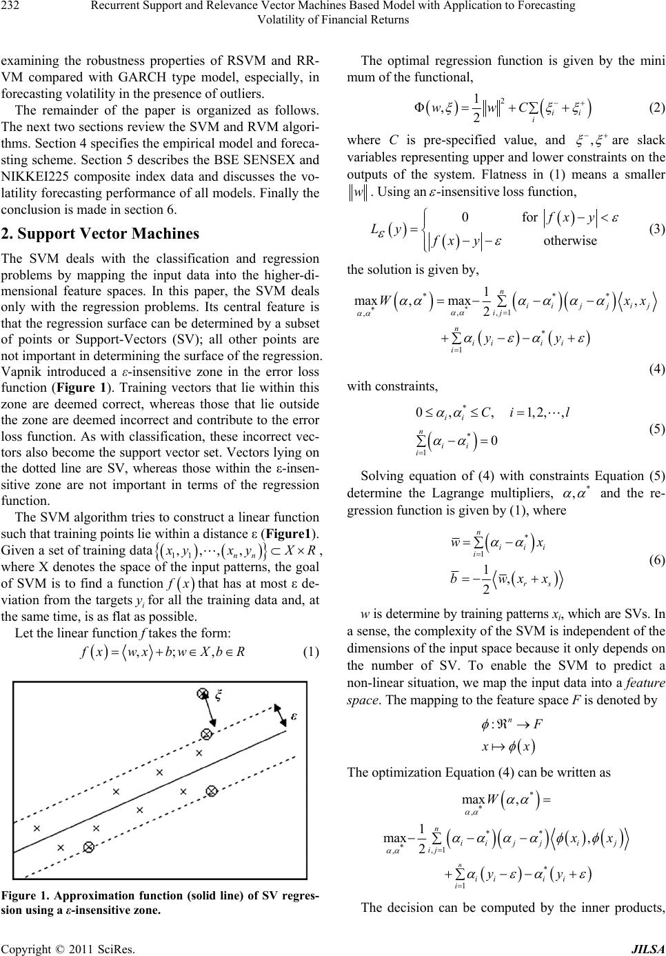

Recurrent Support and Relevance Vector Machines Based Model with Application to Forecasting

232

Volatility of Financial Returns

examining the robustness properties of RSVM and RR-

VM compared with GARCH type model, especially, in

forecasting volatility in the presence of outliers.

The remainder of the paper is organized as follows.

The next two sections review the SVM and RVM algori-

thms. Section 4 specifies the empirical model and foreca-

sting scheme. Section 5 describes the BSE SENSEX and

NIKKEI225 composite index data and discusses the vo-

latility forecasting performance of all models. Finally the

conclusion is made in section 6.

2. Support Vector Machines

The SVM deals with the classification and regression

problems by mapping the input data into the higher-di-

mensional feature spaces. In this paper, the SVM deals

only with the regression problems. Its central feature is

that the regression surface can be determined by a subset

of points or Support-Vectors (SV); all other points are

not important in determining the surface of the regression.

Vapnik introduced a ε-insensitive zone in the error loss

function (Figure 1). Training vectors that lie within this

zone are deemed correct, whereas those that lie outside

the zone are deemed incorrect and contribute to the error

loss function. As with classification, these incorrect vec-

tors also become the support vector set. Vectors lying on

the dotted line are SV, whereas those within the ε-insen-

sitive zone are not important in terms of the regression

function.

The SVM algorithm tries to construct a linear function

such that training points lie within a distance ε (Figure1).

Given a set of training data







,,,,

yxyX



where X denotes the space of the input patterns, the goal

of SVM is to find a function

xthat has at most ε de-

viation from the targetsifor all the training data and, at

the same time, is as flat as possible.

Let the linear function f takes the form:



,; ,

xwxbwXbR (1)

Figure 1. Approximation function (solid line) of SV regres-

sion using a ε-insensitive zone.

The optimal regression function is given by the mini

mum of the functional,





Φ,2ii

wwC









 

 (2)

where C is pre-specified value, and ,





are slack

variables representing upper and lower constraints on the

outputs of the system. Flatness in (1) means a smaller

w. Using an-insensitive



loss function,

 



0for

otherwise

fx y

Ly fx y















(3)

the solution is given by,

  



*,,1

max ,max,

iij jij

iii i



 

 



 







(4)

with constraints,



0,, 1,2,,

Ci l













(5)

Solving equation of (4) with constraints Equation (5)

determine the Lagrange multipliers, *



and the re-

gression function is given by (1), where



iii

bwxx









 

(6)

w is determine by training patterns xi, which are SVs. In

a sense, the complexity of the SVM is independent of the

dimensions of the input space because it only depends on

the number of SV. To enable the SVM to predict a

non-linear situation, we map the input data into a feature

space. The mapping to the feature space F is denoted by









The optimization Equation (4) can be written as





 





*,1

max ,

iij jij

iii i





 











The decision can be computed by the inner products,

Recurrent Support and Relevance Vector Machines Based Model with Application to Forecasting 233

Volatility of Financial Returns

(),( )



without explicitly mapping to a higher

dimension which is a time-consuming task. Hence the

kernel function is as follows:







xzx z





By using a kernel function, it is possible to compute

the SVM without explicitly mapping in the feature space.

3. Relevance Vector Machines

Let 1i be a training data. The goal is to model

the data by a function indexed by parameters defined as





jjj

yxwwx wx











, (7)

where basis function

 



1,, T

 





is non-

linear, 1mis weight vector and x in input

vector. Hence the target is sum of the function and error

term:



,,ww

ty i



 (8)

and vector form of the target is written as



 (9)

For simplicity, i



are assumed to follow independent

Gaussian process with mean zero and variance2



. The

likelihood of the complete dataset corresponding to (8) is

obtained as the following





2πexp 2

ptwN y























For the n simultaneously training points,





,2πexp 2

2πexp ,

iii

ptwt y

 



































(10)

where ,and is (n × m)

design matrix with nand

. As [46], to avoid

overfitting problems which may be caused by the Maxi-

mum likelihood estimation of w and σ2, zero mean Gaus-

sian prior over the weights w is introduced,



1,,T

tt t

 

1,, ,

xKx



1,, T

ww w



1,,x

 



 

,, T

xKxx























00,

iii

Pw Nw













(11)

where αi is the ith element of vector hyperparameter α

assigned to each model parameter wi.

By Bayes rule,







The posterior in (12) cannot calculated directly as de-

nominator of (12) contain normalizing integral i.e.,







 

,,,,dddPt PtwPww2









However, the posterior can be decomposed as









,,,, ,



wtPwtP

 

t

(13)

Now, the first term of (13) can be written as below



,, ,

Ptw Pw

Pwt Pt





 

.

Noticeably,







,,PtPtw Pww

 

dis con-

volution of Gaussians,







is Gaussian prior and





,Ptw



is also Gaussian likelihood by (10), imply-

ing the posterior





,,Pwt





is Gaussian which ob-

tained as [47],









111

2πexp 2

Pwt























(14)

with covariance



2ΦΦ







 (15)

and mean

1ΦTt





 (16)

where





diag, , ,





.

In order to evaluate



and we need to find the

hyperparameters





and 2



which maximize the second

term of (13):











,,PtPtPP



  

For uniform hyperprior, it is just required to maximize

the term







with respect to



and 2



ignoring







and







. Then, the problem becomes













2,, ,,

,, Ptw Pw

Pw tPt







 (12)



,,d

2πΦΦ

expΦΦ .

PtPtw Pww

tIAt

 



























(17)

This is called marginal likelihood which needs to

maximize with respect to



and2



. The maximization

process is known as type II maximum likelihood method

or evidence procedure. The hyperparameters are esti-

mated by iterative method as it cannot be obtained in

closed form.

As from [30], the solutions are obtained,

new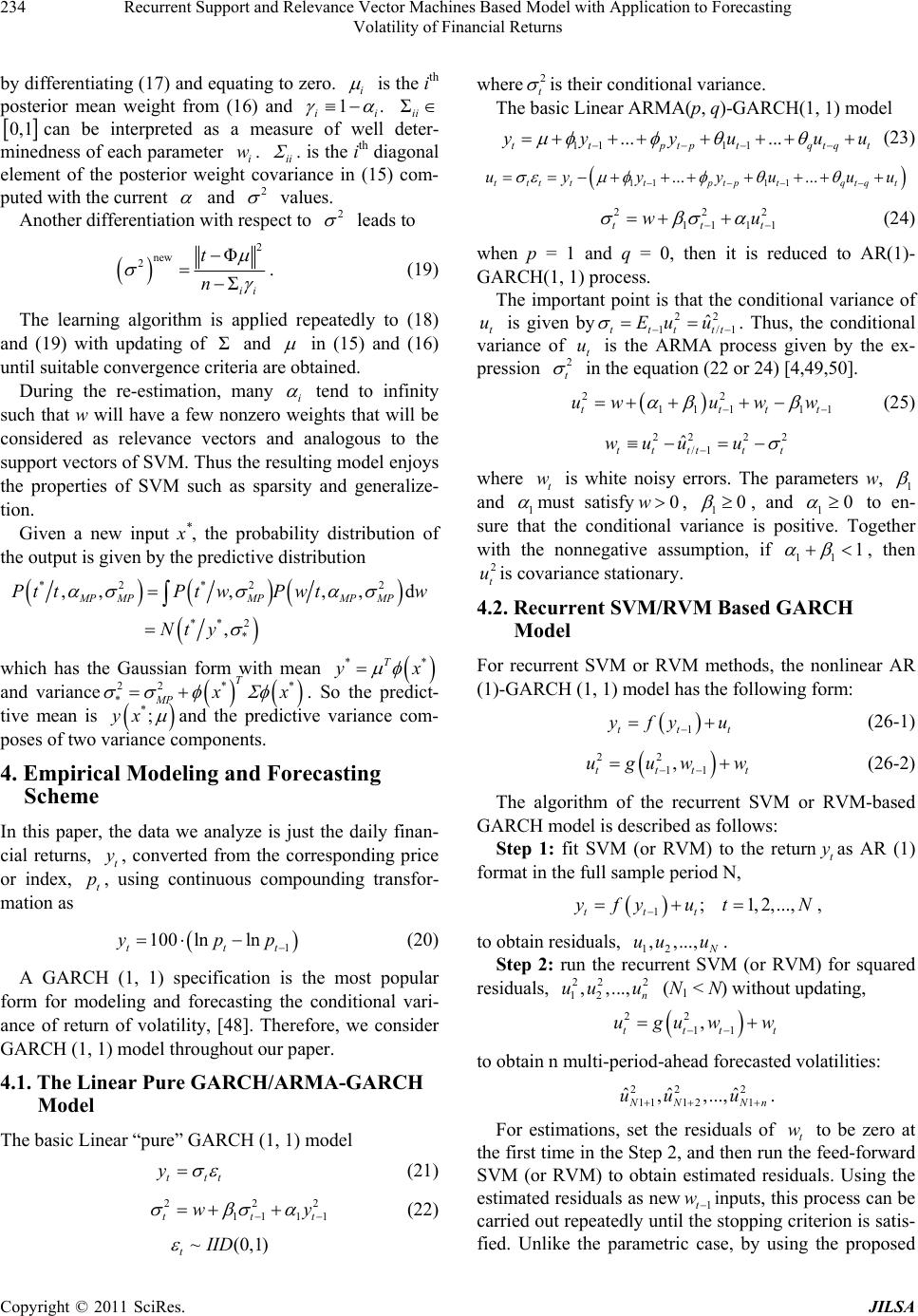







 (18)

Recurrent Support and Relevance Vector Machines Based Model with Application to Forecasting

234

Volatility of Financial Returns

by differentiating (17) and equating to zero. i



is the ith

posterior mean weight from (16) and 1.





 Σii







0,1 can be interpreted as a measure of well deter-

minedness of each parameter i. ii. is the ith diagonal

element of the posterior weight covariance in (15) com-

puted with the current





and 2



values.

Another differentiation with respect to 2



leads to



new

2Φ

Σii









. (19)

The learning algorithm is applied repeatedly to (18)

and (19) with updating of and



in (15) and (16)

until suitable convergence criteria are obtained.

During the re-estimation, many i



tend to infinity

such that w will have a few nonzero weights that will be

considered as relevance vectors and analogous to the

support vectors of SVM. Thus the resulting model enjoys

the properties of SVM such as sparsity and generalize-

tion.

Given a new input x*, the probability distribution of

the output is given by the predictive distribution





*2 *22

**2

,,,,,d

MP MPMPMP MP

Pt tPtwPwtw

Nt y









which has the Gaussian form with mean







*

and variance



22 **

 





*;yx

. So the predict-

tive mean is



and the predictive variance com-

poses of two variance components.

4. Empirical Modeling and Forecasting

Scheme

In this paper, the data we analyze is just the daily finan-

cial returns, t, converted from the corresponding price

or index, , using continuous compounding transfor-

mation as



100 lnln





  (20)

A GARCH (1, 1) specification is the most popular

form for modeling and forecasting the conditional vari-

ance of return of volatility, [48]. Therefore, we consider

GARCH (1, 1) model throughout our paper.

4.1. The Linear Pure GARCH/ARMA-GA RCH

Model

The basic Linear “pure” GARCH (1, 1) model





 (21)

11 11tt





 2



)

(22)

~(0,1

tIID



where 2



is their conditional variance.

The basic Linear ARMA(p, q)-GARCH(1, 1) model

11 11

... ...

ttptptqtqt

yyuu

 





 

(23)





11 11

... ...

tttttptptqtqt

uyy yuu





  u



11 11tt





 (24)

when p = 1 and q = 0, then it is reduced to AR(1)-

GARCH(1, 1) process.

The important point is that the conditional variance of

t is given by1

u22

ttttt

Eu u





. Thus, the conditional

variance of t is the ARMA process given by the ex-

pression



in the equation (22 or 24) [4,49,50].





111 1ttt

uwu ww

 



 



(25)

22 2

ttttt

wuu u









where is white noisy errors. The parameters w,



and 1



must satisfy, 1

0w0



, and 10





to en-

sure that the conditional variance is positive. Together

with the nonnegative assumption, if



, then

is covariance stationary.

4.2. Recurrent SVM/RVM Based GARCH

Model

For recurrent SVM or RVM methods, the nonlinear AR

(1)-GARCH (1, 1) model has the following form:





1ttt

fy u





 (26-1)





ttt

uguw w

 t



 (26-2)

The algorithm of the recurrent SVM or RVM-based

GARCH model is described as follows:

Step 1: fit SVM (or RVM) to the returnas AR (1)

format in the full sample period N,





1; 1,2,...,

ttt

fyutN



,

to obtain residuals, 12

, ,...,

uu u.

Step 2: run the recurrent SVM (or RVM) for squared

residuals, (

N1 < N) without updating,

22 2

,,..., n

uu u





ttt

uguw w

 t





to obtain n multi-period-ahead forecasted volatilities:

22 2

11 121

ˆˆ ˆ

, ,...,

uuu





For estimations, set the residuals of t to be zero at

the first time in the Step 2, and then run the feed-forward

SVM (or RVM) to obtain estimated residuals. Using the

estimated residuals as new1tinputs, this process can be

carried out repeatedly until the stopping criterion is satis-

fied. Unlike the parametric case, by using the proposed

w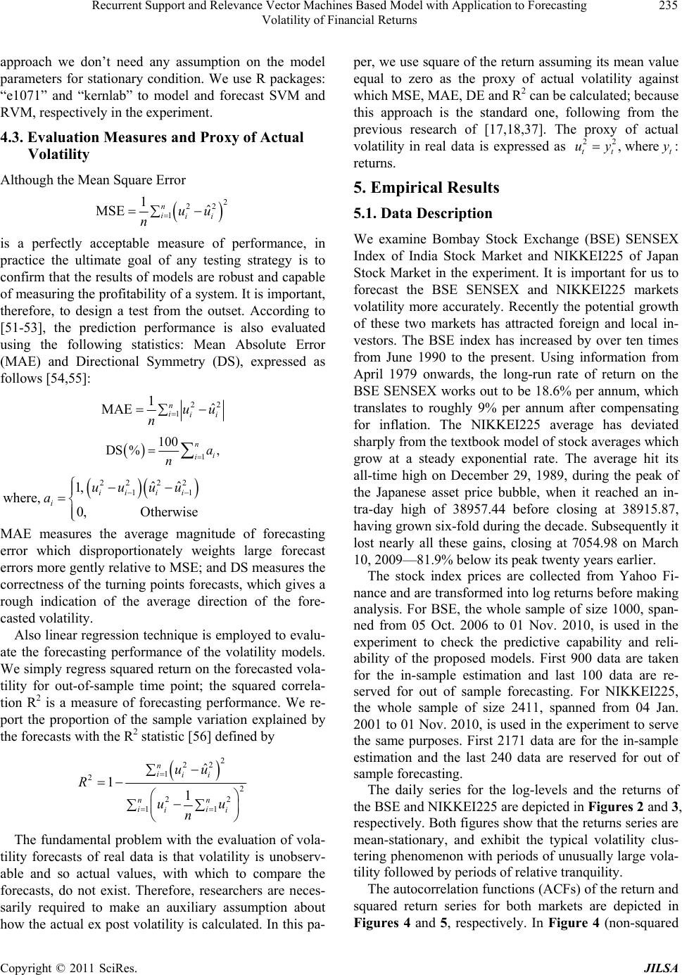

Recurrent Support and Relevance Vector Machines Based Model with Application to Forecasting 235

Volatility of Financial Returns

approach we don’t need any assumption on the model

parameters for stationary condition. We use R packages:

“e1071” and “kernlab” to model and forecast SVM and

RVM, respectively in the experiment.

4.3. Evaluation Measures and Proxy of Actual

Volatility

Although the Mean Square Error



1ˆ

MSE n

iii

n





is a perfectly acceptable measure of performance, in

practice the ultimate goal of any testing strategy is to

confirm that the results of models are robust and capable

of measuring the profitability of a system. It is important,

therefore, to design a test from the outset. According to

[51-53], the prediction performance is also evaluated

using the following statistics: Mean Absolute Error

(MAE) and Directional Symmetry (DS), expressed as

follows [54,55]:

1ˆ

MAE n

iii

n







100

DS %,

n





2222

ˆˆ

where, 0, Otherwise

ii ii

uu uu

a











MAE measures the average magnitude of forecasting

error which disproportionately weights large forecast

errors more gently relative to MSE; and DS measures the

correctness of the turning points forecasts, which gives a

rough indication of the average direction of the fore-

casted volatility.

Also linear regression technique is employed to evalu-

ate the forecasting performance of the volatility models.

We simply regress squared return on the forecasted vola-

tility for out-of-sample time point; the squared correla-

tion R2 is a measure of forecasting performance. We re-

port the proportion of the sample variation explained by

the forecasts with the R2 statistic [56] defined by



iii









 









The fundamental problem with the evaluation of vola-

tility forecasts of real data is that volatility is unobserv-

able and so actual values, with which to compare the

forecasts, do not exist. Therefore, researchers are neces-

sarily required to make an auxiliary assumption about

how the actual ex post volatility is calculated. In this pa-

per, we use square of the return assuming its mean value

equal to zero as the proxy of actual volatility against

which MSE, MAE, DE and R2 can be calculated; because

this approach is the standard one, following from the

previous research of [17,18,37]. The proxy of actual

volatility in real data is expressed as where :

returns.

uyt

5. Empirical Results

5.1. Data Description

We examine Bombay Stock Exchange (BSE) SENSEX

Index of India Stock Market and NIKKEI225 of Japan

Stock Market in the experiment. It is important for us to

forecast the BSE SENSEX and NIKKEI225 markets

volatility more accurately. Recently the potential growth

of these two markets has attracted foreign and local in-

vestors. The BSE index has increased by over ten times

from June 1990 to the present. Using information from

April 1979 onwards, the long-run rate of return on the

BSE SENSEX works out to be 18.6% per annum, which

translates to roughly 9% per annum after compensating

for inflation. The NIKKEI225 average has deviated

sharply from the textbook model of stock averages which

grow at a steady exponential rate. The average hit its

all-time high on December 29, 1989, during the peak of

the Japanese asset price bubble, when it reached an in-

tra-day high of 38957.44 before closing at 38915.87,

having grown six-fold during the decade. Subsequently it

lost nearly all these gains, closing at 7054.98 on March

10, 2009—81.9% below its peak twenty years earlier.

The stock index prices are collected from Yahoo Fi-

nance and are transformed into log returns before making

analysis. For BSE, the whole sample of size 1000, span-

ned from 05 Oct. 2006 to 01 Nov. 2010, is used in the

experiment to check the predictive capability and reli-

ability of the proposed models. First 900 data are taken

for the in-sample estimation and last 100 data are re-

served for out of sample forecasting. For NIKKEI225,

the whole sample of size 2411, spanned from 04 Jan.

2001 to 01 Nov. 2010, is used in the experiment to serve

the same purposes. First 2171 data are for the in-sample

estimation and the last 240 data are reserved for out of

sample forecasting.

The daily series for the log-levels and the returns of

the BSE and NIKKEI225 are depicted in Figures 2 and 3,

respectively. Both figures show that the returns series are

mean-stationary, and exhibit the typical volatility clus-

tering phenomenon with periods of unusually large vola-

tility followed by periods of relative tranquility.

The autocorrelation functions (ACFs) of the return and

squared return series for both markets are depicted in

Figures 4 and 5, respectively. In Figure 4 (non-squared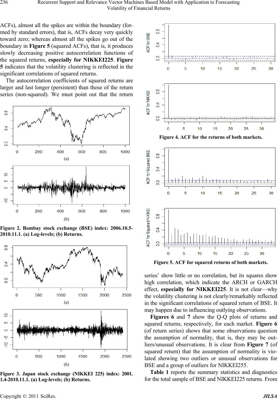

Recurrent Support and Relevance Vector Machines Based Model with Application to Forecasting

236

Volatility of Financial Returns

ACFs), almost all the spikes are within the boundary (for-

med by standard errors), that is, ACFs decay very quickly

toward zero; whereas almost all the spikes go out of the

boundary in Figure 5 (squared ACFs), that is, it produces

slowly decreasing positive autocorrelation functions of

the squared returns, especially for NIKKEI225. Figure

5 indicates that the volatility clustering is reflected in the

significant correlations of squared returns.

The autocorrelation coefficients of squared returns are

larger and last longer (persistent) than those of the return

series (non-squared). We must point out that the return

(a)

(b)

Figure 2. Bombay stock exchange (BSE) index: 2006.10.5-

2010.11.1. (a) Log-levels; (b) Returns.

(a)

(b)

Figure 3. Japan stock exchange (NIKKEI 225) index: 2001.

1.4-2010.11.1. (a) Log-levels; (b) Returns.

Figure 4. ACF for the returns of both markets.

Figure 5. ACF for squared returns of both markets.

series’ show little or no correlation, but its squares show

high correlation, which indicate the ARCH or GARCH

effect, especially for NIKKEI225. It is not clear—why

the volatility clustering is not clearly/remarkably reflected

in the significant correlations of squared return of BSE. It

may happen due to influencing outlying observations.

Figures 6 and 7 show the Q-Q plots of returns and

squared returns, respectively, for each market. Figure 6

(of return series) shows that some observations question

the assumption of normality, that is, they may be out-

liers/unusual observations. It is clear from Figure 7 (of

squared return) that the assumption of normality is vio-

lated showing two outliers or unusual observations for

BSE and a group of outliers for NIKKEI255.

Table 1 reports the summary statistics and diagnostics

for the total sample of BSE and NIKKEI225 returns. From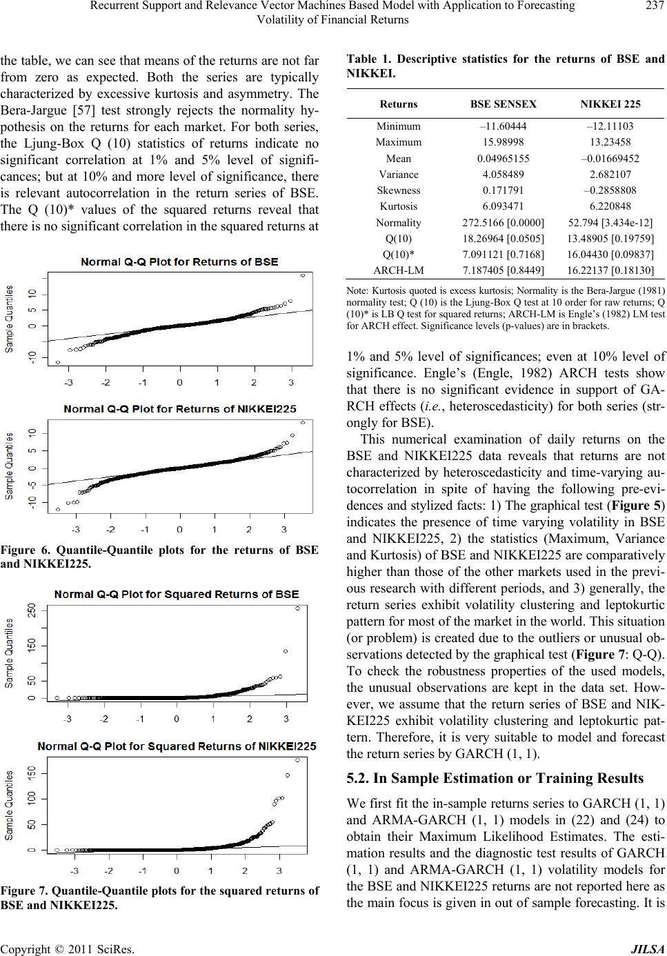

Recurrent Support and Relevance Vector Machines Based Model with Application to Forecasting 237

Volatility of Financial Returns

the table, we can see that means of the returns are not far

from zero as expected. Both the series are typically

characterized by excessive kurtosis and asymmetry. The

Bera-Jargue [57] test strongly rejects the normality hy-

pothesis on the returns for each market. For both series,

the Ljung-Box Q (10) statistics of returns indicate no

significant correlation at 1% and 5% level of signifi-

cances; but at 10% and more level of significance, there

is relevant autocorrelation in the return series of BSE.

The Q (10)* values of the squared returns reveal that

there is no significant correlation in the squared returns at

Figure 6. Quantile-Quantile plots for the returns of BSE

and NIKKEI225.

Figure 7. Quantile-Quantile plots for the squared retur ns of

BSE and NIKKEI225.

Table 1. Descriptive statistics for the returns of BSE and

NIKKEI.

Returns BSE SENSEX NIKKEI 225

Minimum –11.60444 –12.11103

Maximum 15.98998 13.23458

Mean 0.04965155 –0.01669452

Variance 4.058489 2.682107

Skewness 0.171791 –0.2858808

Kurtosis 6.093471 6.220848

Normality 272.5166 [0.0000] 52.794 [3.434e-12]

Q(10) 18.26964 [0.0505] 13.48905 [0.19759]

Q(10)* 7.091121 [0.7168] 16.04430 [0.09837]

ARCH-LM 7.187405 [0.8449] 16.22137 [0.18130]

Note: Kurtosis quoted is excess kurtosis; Normality is the Bera-Jargue (1981)

normality test; Q (10) is the Ljung-Box Q test at 10 order for raw returns; Q

(10)* is LB Q test for squared returns; ARCH-LM is Engle’s (1982) LM test

for ARCH effect. Significance levels (p-values) are in brackets.

1% and 5% level of significances; even at 10% level of

significance. Engle’s (Engle, 1982) ARCH tests show

that there is no significant evidence in support of GA-

RCH effects (i.e., heteroscedasticity) for both series (str-

ongly for BSE).

This numerical examination of daily returns on the

BSE and NIKKEI225 data reveals that returns are not

characterized by heteroscedasticity and time-varying au-

tocorrelation in spite of having the following pre-evi-

dences and stylized facts: 1) The graphical test (Figure 5)

indicates the presence of time varying volatility in BSE

and NIKKEI225, 2) the statistics (Maximum, Variance

and Kurtosis) of BSE and NIKKEI225 are comparatively

higher than those of the other markets used in the previ-

ous research with different periods, and 3) generally, the

return series exhibit volatility clustering and leptokurtic

pattern for most of the market in the world. This situation

(or problem) is created due to the outliers or unusual ob-

servations detected by the graphical test (Figure 7: Q-Q).

To check the robustness properties of the used models,

the unusual observations are kept in the data set. How-

ever, we assume that the return series of BSE and NIK-

KEI225 exhibit volatility clustering and leptokurtic pat-

tern. Therefore, it is very suitable to model and forecast

the return series by GARCH (1, 1).

5.2. In Sample Estimation or Training Results

We first fit the in-sample returns series to GARCH (1, 1)

and ARMA-GARCH (1, 1) models in (22) and (24) to

obtain their Maximum Likelihood Estimates. The esti-

mation results and the diagnostic test results of GARCH

(1, 1) and ARMA-GARCH (1, 1) volatility models for

the BSE and NIKKEI225 returns are not reported here as

the main focus is given in out of sample forecasting. It is

Recurrent Support and Relevance Vector Machines Based Model with Application to Forecasting

Volatility of Financial Returns

238

seen that based on log likelihood (LL), AIC, and BIC

criteria, ARMA-GARCH (1, 1) model is more adequate

to the data than pure GARCH (1, 1) model.

Now we turn to consider our models, recurrent support

vector machine and recurrent relevance vector machine.

The considered models must be trained using the above

algorithm stated in Step 1 and Step 2. While training

RSVM, two parameters



and Care considered since they

are sensitive for modeling the SVM.



is assumed to be

0.005 and used for all cases. We apply ten-fold-cross-va-

lidation technique to tune the values of



and with the

range [2–5, 25] and [2–5, 25], respectively. The optimal

parameters







= (22, 2–2) and (25, 22) for training

BSE and NIKKEI225, respectively. Table 2 illustrates

the training results (only the number of support vectors

and relevance vectors) by RSVM and RRVM for both

markets. From the Table 2, we can see that RRVM is

more adequate to the in-sample series compared to

RSVM for each market since RRVM produces smallest

number of relevance vectors compared to the number of

support vectors of RSVM.

5.3. Out of Sample Volatility Forecasting Results

Table 3 summarizes the forecasting performance based

on four measures defined in section 4.3, MSE, MAE, DS

and R square. From the table 3, we can see that ARMA-

GARCH generates smaller values of SqrtMSE (3.1742)

and MAE (3.0199) but larger value of R2 (0.00553) than

those of pure GARCH for BSE. For NIKKEI225, ARMA-

GARCH generates smaller values of SqrtMSE (2.8094)

and MAE (2.2401) than those of pure GARCH. Both the

ARMA-GARCH and pure GARCH produce the same

value of DS for each market and R2 for NIKKEI225.

Hence the ARMA-GARCH model outperforms the pure

GARCH model.

Whereas RSVM and RRVM, they provide better per-

formance than GARCH type models (pure GARCH and

ARMA-GARCH) for all cases except the RSVM for NI-

KKEI225 based on MSE and DS, where GARCH type

models perform better than RSVM. If we make compa-

rison between RSVM and RRVM, the RSVM is better

than RRVM based on MAE and R2 only; but in term of

MSE and DS, the RRVM is better than RSVM for both

markets. The forecasting performances of GARCH type

models are very poor compared to that of RSVM and

RRVM due to outliers affect on traditional GARCH type

model in forecasting; that is, both the RSVM and RRVM

(not GARCH type) hold the robustness properties in for-

ecasting through estimation.

Figures 8 and 9 plot multi-period-ahead forecasts by

the machine learning models (RSVM and RRVM) and

GARCH type models (pure GARCH and ARMA-GAR-

Table 2. Training results for RSVM and RRVM.

BSE NIKKEI225

No. of S.V.s 661 2049

No. of R.V.s 77 49

Figure 8. Volatility forecasts of BSE index returns.

Table 3. Multi-period-ahead forecasting accuracy by different models for real data.

BSE NIKKEI225

Models

Sqrt MSE MAE DS R2 Sqrt MSEMAE DS R2

GARCH 3.2568 3.1024 51 0.00485 2.8124 2.2464 52.5 0.00071

ARMA-GARCH 3.1742 3.0199 51 0.00553 2.8094 2.2401 52.5 0.00071

RSVM 1.1160

0.6258 65 0.03011 3.0073 1.6864 50.4 0.00417

RRVM 1.0670 0.8104 87 0.02973 2.7466 1.7677 95.8 4.58E-5

Recurrent Support and Relevance Vector Machines Based Model with Application to Forecasting 239

Volatility of Financial Returns

Figure 9. Volatility forecasts of NIKKEI225 index returns.

CH) against actual values for BSE and NIKKEI225, re-

spectively. From the plots we can see that the machine

learning techniques generate better forecasting perform-

ances than the GARCH type models. The forecasted se-

ries’ by GARCH type models are pushed up due to outli-

ers affect; where the ARMA-GARCH model is less af-

fected than pure GARCH. The series by RSVM is not

affected due to its robustness properties; where RRVM is

slightly affected by outliers for BSE. For NIKKEI, no

model is remarkably affected by outliers; because of hav-

ing a group of outliers which may not be very much in-

fluential.

6. Conclusions

To measure the model performances, we apply recurrent

SVM and RVM to model GARCH as hybrid approaches

comparing with traditional pure GARCH and ARMA-

GARCH models to forecast (multi-periodically) volatility

of Asian (emerging) stock markets, BSE SENSEX and

NIKKEI225. The above models are evaluated using the

criteria: MSE, MAE, DS and linear regression R2 in out-

of-sample forecasting. In the parallel way, we examine

the robustness properties of the used models in forecast-

ing volatility in the presence of outliers, where outliers

are detected very simply using Q-Q plot. Using Q-Q pl-

ots of the observed volatility, two outliers are clearly de-

tected for BSE and a group of outliers for NIKKEI225.

Due to the affect of these outliers, the ACFs (especially,

of BSE), descriptive statistics and classical tests (Ljung-

Box Q and ARCH-LM) give the misleading results, wh-

ich agree with the previous research on outliers in time

series analysis. From the experimental results, we can

come to the conclusion that 1) the outliers significantly

affect the parameter estimates of the pure GARCH and

ARMA-GARCH models, 2) the RRVM produces small-

lest number of relevance vectors compared to the number

of support vectors of RSVM, 3) the computational-in-

telligence-based techniques (RSVM and RRVM) per-

form better than the GARCH type models in out-of-sam-

ple forecasting, 4) the ARMA-GARCH model is superior

to the pure GARCH model in out-of-sample forecasting,

5) both the RSVM and RRVM perform almost equally in

out-of-sample forecasting—the RSVM is better than

RRVM based on MAE and R2, but in terms of MSE and

DS, the RRVM is better than RSVM, and 6) RRVM with

RSVM holds the robustness properties in forecasting

through estimation, however, RRVM is slightly affected

by outliers for being Bayesian approach. Theoretically,

RVM is a probabilistic model having its functional form

identical to SVM, where there is no requirement of free

parameters and Mercer’s kernel function for RVM like

SVM. Considering the above empirical results and theo-

retical properties of RVM and SVM, we are in favor of

recurrent RVM (like the previous research) in forecasting

volatility of emerging stock markets, even in the pres-

ence of outliers.

REFERENCES

[1] R. F. Engle and A. J. Patton, “What Good Is a Volatility

Model?” Journal of Quantitative Finance, Vol. 1, No. 2,

2001, pp. 237-245. doi:10.1088/1469-7688/1/2/305

[2] R. C. Merton, “On Estimating the Expected Return on the

Market: An Exploratory Investigation,” Journal of Fi-

nancial Economics, Vol. 8, 1980, pp. 323-361.

doi:10.1016/0304-405X(80)90007-0

[3] R. F. Engle, “Autoregressive Conditional Heteroscedas-

ticity with Estimates of the Variance of United Kingdom

Inflation,” Econometrica, Vol. 50, No. 2, 1982, pp. 987-

1007. doi:10.2307/1912773

[4] T. Bollerslev, “Generalized Autoregressive Conditional He-

teroscedasticity,” Journal of Econometric, Vol. 31, No. 3,

1986, pp. 307-327. doi:10.1016/0304-4076(86)90063-1

[5] S. H. Poon and C. Granger, “Forecasting Volatility in Fi-

nancial Markets: A Review,” Journal of Economic Lit-

erature, Vol. 41, No. 2, 2003, pp. 478-539.

doi:10.1257/002205103765762743

[6] W. C. Wong, F. Yip and L. Xu, “Financial Prediction by

Finite Mixture GARCH Model,” Proceedings of Fifth In-

ternational Conference on Neural Information Processing,

Kitakyushu, 21-23 October 1998, pp. 1351-1354.

[7] H. Tang, K. C. Chun and L. Xu, “Finite Mixture of

ARMA-GARCH Model for Stock Price Prediction,” Pro-

ceedings of 3rd International Workshop on Computatio-

nal Intelligence in Economics and Finance (CIEF 2003),

North Carolina, 26-30 September 2003, pp. 1112-1119.

[8] A. Hossain and M. Nasser, “Comparison of Finite Mix-

ture of ARMA-GARCH, Back Propagation Neural Net-

works and Support-Vector Machines in Forecasting Fi-

nancial Returns,” Journal of Applied Statistics, Vol. 38,

Recurrent Support and Relevance Vector Machines Based Model with Application to Forecasting

240

Volatility of Financial Returns

No. 3, 2011, pp. 533-551.

[9] T. G. Andersen and T. Bollerslev, “Answering the Skep-

tics: Yes, Standard Volatility Models Do Provide Accu-

rate Forecasts,” International Economic Review, Vol. 39,

No. 4, 1998, pp. 885-905. doi:10.2307/2527343

[10] T. J. Brailsford and R. W. Faff, “An Evaluation of Vola-

tility Forecasting Techniques,” Journal of Banking and

Finance, Vol. 20, No. 3, 1996, pp. 419-438.

doi:10.1016/0378-4266(95)00015-1

[11] R. Cumby, S. Figlewski and J. Hasbrouck, “Forecasting

Volatility and Correlations with EGARCH Models,” Jour-

nal of Derivatives Winter, Vol. 1, No. 2, 1993, pp. 51-63.

[12] S. Figlewski, “Forecasting Volatility,” Financial Markets,

Institutions and Instruments, Vol. 6, No. 1, 1997, pp. 1-88.

doi:10.1111/1468-0416.00009

[13] P. Jorion, “Predicting Volatility in the Foreign Exchange

Market,” Journal of Finance, Vol. 50, No. 2, 1995, pp.

507-528. doi:10.2307/2329417

[14] P. Jorion, “Risk and Turnover in the Foreign Exchange

Market,” In: J. A. Franke, G. Galli and A. Giovannini,

Eds., The Microstructure of Foreign Exchange Markets,

Chicago University Press, Chicago, 1996.

[15] D. G. McMillan, A. E. H. Speight and O. Gwilym, “Fore-

casting UK Stock Market Volatility: A Comparative Ana-

lysis of Alternate Methods,” Applied Financial Econom-

ics, Vol. 10, No. 4, 2000, pp. 435-448.

doi:10.1080/09603100050031561

[16] R. G. Donaldson and M. Kamstra, “An Artificial Neural

Network-GARCH Model for International Stock Returns

Volatility,” Journal of Empirical Finance, Vol. 4, No. 1,

1997, pp. 17-46. doi:10.1016/S0927-5398(96)00011-4

[17] F. Perez-Cruz, J. A. Afonso-Rodriguez and J. Giner, “Es-

timating GARCH Models Using Support Vector Machi-

nes,” Journal of Quantitative Finance, Vol. 3, 2003, pp.

163-172.

[18] P. H. Ou and H. Wang, “Predicting GARCH, EGARCH,

GJR Based Volatility by the Relevance Vector Machine:

Evidence from the Hang Seng Index,” International Re-

search Journal of Finance and Economics, No. 39, 2010,

pp. 46-63.

[19] L. B. Tang, H. Y. Sheng and L. X. Tang, “Forecasting Vo-

latility Based on Wavelet Support Vector Machine,” Ex-

pert Systems with Applications, Vol. 36, No. 2, 2009, pp.

2901-2909.

[20] L. B. Tang, H. Y. Sheng and L. X. Tang, “GARCH Pre-

diction Using Spline Wavelet Support Vector Machine,”

Journal of Neural Computing and Application, Vol. 18,

No. 8, 2009, pp. 913-917.

[21] M. Bildirici and Ö. Ö. Ersin, “Improving Forecasts of

GARCH Family Models with the Artificial Neural Net-

works: An Application to the Daily Returns in Istanbul

Stock Exchange,” Expert Systems with Applications, Vol.

36, No. 4, 2009, pp. 7355-7362.

doi:10.1016/j.eswa.2008.09.051

[22] L. J. Cao and F. Tay, “Application of Support Vector

Machines in Financial Time Series Forecasting,” Interna-

tional Journal of Management Science, Vol. 29, No. 4,

2001, pp. 309-317.

[23] V. N. Vapnik, “The Nature of Statistical Learning The-

ory,” 2nd Edition, Sringer-Verlag, New York, 1995.

[24] L. J. Cao and F. Tay, “Modified Support Vector Machines

in Financial Time Series Forecasting,” Journal of Neuro-

computing, Vol. 48, No. 1-4, 2002, pp. 847-861.

[25] K. J. Kim, “Financial Time Series Forecasting Using Sup-

port Vector Machines,” Journal of Neurocomputing, Vol.

55, No. 1-2, 2003, pp. 307-319.

[26] W. Huang, Y. Nakamori and S. Y. Wang, “Forecasting

Stock Market Movement Direction with Support Vector

Machine,” Journal of Computers & Operational Re-

search, Vol. 32, No. 10, 2005, pp. 513-522.

[27] C. J. Lu, T. S. Lee and C. C. Chiu, “Financial Time Series

Forecasting Using Independent Component Analysis and

Support Vector Regression,” Journal of Decision Support

Systems, Vol. 47, No. 2, 2009, pp. 115-125.

[28] H. S. Kim and S. Y. Sohn, “Support Vector Machines for

Default Prediction of SMEs Based on Technology Credit,”

European Journal of Operational Research, Vol. 201, No.

3, 2010, pp. 938-846.

[29] A. J. Smola and B. Scholkopf, “A Tutorial on Support

Vector Regression,” Journal of Statistics and Computing,

Vol. 14, No. 3, 2004, pp. 199-222.

[30] M. E. Tipping, “Sparse Bayesian Learning and the Rele-

vance Vector Machine,” Journal of Machine Learning

Research, Vol. 1, 2001, pp. 211-244.

[31] C. M. Bishop and M. E. Tipping, “Variational Relevance

Vector Machine,” In: C. Boutilier and M. Goldszmidt,

Eds., Uncertainty in Artificial Intelligence, Morgan Kau-

fmann, Waltham, 2000, pp. 46-53.

[32] S. Ghosh and P. P. Mujumdar, “Statistical Downscaling

of GCM Simulations to Stream Flow Using Relevance

Vector Machine,” Advances in Water Resources, Vol. 31,

No. 1, 2008, pp. 132-146.

[33] D. Porro, N. Hdez, I. Talavera, O. Nunez, A. Dago and R.

J. Biscay, “Performance Evaluation of Relevance Vector

Machines as a Nonlinear Regression method in Real

World Chemical Spectroscopic Data,” 19th International

Conference on Pattern Recognition (ICPR 2008), Tampa,

8-11 December 2008, pp. 1-4.

[34] S. Chen, K. Jeong and W. Härdle, “Support Vector Regres-

sion Based GARCH Model with Application to Forecast-

ing Volatility of Financial Returns,” SFB 649 Discussion

Paper 2008-014.

http://edoc.hu-berlin.de/series/sfb-649-papers/2008-14/PD

F/14.pdf

[35] S. Chen, K. Jeong and W. Härdle, “Recurrent Support

Vector Regression for a Nonlinear ARMA Model with

Applications to Forecasting Financial Returns,” SFB 649

Discussion Paper 2008-051.

[36] J. A. K. Suykens and J. Vandewalle, “Recurrent Least

Squares Support Vector Machines,” IEEE Transactions

on Circuits and Systems I, Vol. 47, No. 7, 2000, pp. 1109-

1114. doi:10.1109/81.855471

Recurrent Support and Relevance Vector Machines Based Model with Application to Forecasting

Volatility of Financial Returns

241

[37] P. H. Ou and H. Wang, “Predict GARCH Based Volatil-

ity of Shanghai Composite Index by Recurrent Relevant

Vector Machines and Recurrent Least Square Support

Vector Machines,” Journal of Mathematics Research, Vol.

2, No. 2, 2010.

[38] G. Bekaert and C. R. Harvey, “Emerging Equity Market

Volatility,” Journal of Financial Economics, Vol. 43, No.

1, 1997, pp. 29-78. doi:10.1016/S0304-405X(96)00889-6

[39] R. Aggarwal, C. Inclan and R. Leal, “Volatility in Emerg-

ing Stock Markets,” Journal of Financial and Quantita-

tive Analysis, Vol. 34, No. 1, 1999, pp. 33-55.

doi:10.2307/2676245

[40] J. Ledolter, “The Effects of Additive Outliers on the Fore-

casts from ARIMA Models,” International Journal of

Forecasting, Vol. 5, No. 2, 1989, pp. 231-240.

doi:10.1016/0169-2070(89)90090-3

[41] R. F. Engle and G. G. J. Lee, “A Permanent and Transi-

tory Component Model of Stock Returns Volatility,” Dis-

cussion Paper 92-44R, University of California, San Die-

go, 1993.

[42] P. H. Franses, D. van Dijk and A. Locas, “Short Patches

of Outliers, ARCH and Volatility Modeling,” Discussion

Paper 98-057/4, Tinbergen Institute, Erasmus University,

Rotterdam, 1998.

[43] P. H. Franses and H. Ghijsels, “Additive Outliers, GARCH

and Forecasting Volatility,” International Journal of Fore-

casting, Vol. 15, No. 1, 1999, pp. 1-9.

doi:10.1016/S0169-2070(98)00053-3

[44] A. J. Fox, “Outliers in Time Series,” Journal of the Royal

Statistical Society, Series B, Vol. 34, No. 3, 1972, pp. 350-

363.

[45] C. Chen and L. Liu, “Joint Estimation of Model Parame-

ters and Outlier Effects in Time Series,” Journal of Ame-

rican Statistical Association, Vol. 88, No. 421, 1993, pp.

284-297. doi:10.2307/2290724

[46] M. E. Tipping, “Relevance Vector Machine,” Microsoft

Research, Cambridge, 2000.

[47] M. E. Tipping, “Bayesian Inference: An Introduction to

Principles and Practice in Machine Learning,” Advanced

Lectures on Machine Learning, Vol. 3176/2004, 2004, pp.

41-62. doi:10.1007/978-3-540-28650-9_3

[48] P. R. Hansen and A. Lunde, “A Forecast Comparison of

Volatility Models: Does Anything Beat a GARCH (1, 1)?”

Journal of Applied Econometrics, Vol. 20, No. 7, 2005, pp.

873-889.

[49] J. D. Hamilton, “Time Series Analysis,” Princeton Uni-

versity Press, Saddle River, 1997.

[50] W. Enders, “Applied Econometric Time Series,” 2nd Edi-

tion, John Wiley & Sons, New York, 2004.

doi:10.1016/S0305-0483(01)00026-3

[51] F. E. H. Tay and L. Cao, “Application of Support Vector

Machines in Financial Time-Series Forecasting,” Omega,

Vol. 29, No. 4, 2001, pp. 309-317.

[52] M. Thomason, “The Practitioner Method and Tools: A

Basic Neural Network-Based Trading System Project Re-

visited (Parts 1 and 2),” Journal of Computational Intel-

ligence in Finance, Vol. 7, No. 3, 1999, pp. 36-45.

[53] M. Thomason, “The Practitioner Method and Tools: A

Basic Neural Network-Based Trading System Project Re-

visited (Parts 3 and 4),” Journal of Computational Intel-

ligence in Finance, Vol. 7, No. 3, 1999, pp. 35-48.

[54] C. Brooks, “Predicting Stock Index Volatility: Can Mar-

ket Volume Help?” Journal of Forecasting, Vol. 17, No.

1, 1998, pp. 59-80.

doi:10.1002/(SICI)1099-131X(199801)17:1<59::AID-FO

R676>3.0.CO;2-H

[55] I. A. Moosa, “Exchange Rate Forecasting: Techniques and

Applications,” Macmillan Press LTD, Lonton, 2000.

[56] H. Theil, “Principles of Econometrics,” Wiley, New York,

1971.

[57] A. K. Bera and C. M. Jarque, “An Efficient Large-Sample

Test for Normality of Observations and Regression Re-

siduals,” Australian National University Working Papers

in Econometrics, 40, Canberra, 1981.