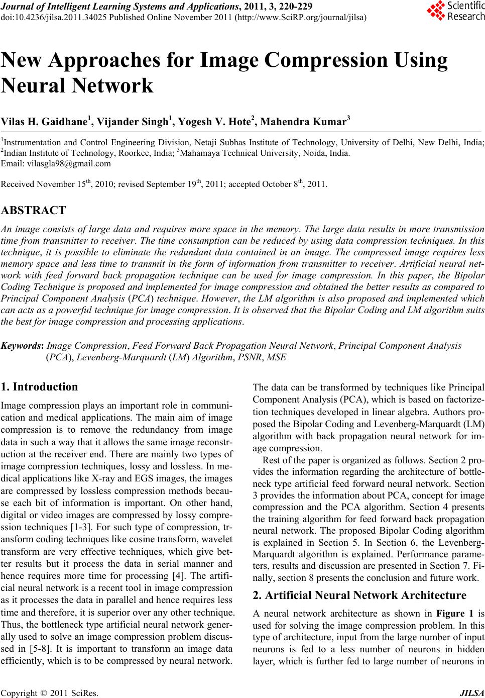
 Journal of Intelligent Learning Systems and Applications, 2011, 3, 220-229 doi:10.4236/jilsa.2011.34025 Published Online November 2011 (http://www.SciRP.org/journal/jilsa) Copyright © 2011 SciRes. JILSA New Approaches for Image Compression Using Neural Network Vilas H. Gaidhane1, Vijander Singh1, Yogesh V. Hote2, Mahendra Kumar3 1Instrumentation and Control Engineering Division, Netaji Subhas Institute of Technology, University of Delhi, New Delhi, India; 2Indian Institute of Technology, Roorkee, India; 3Mahamaya Technical University, Noida, India. Email: vilasgla98@gmail.com Received November 15th, 2010; revised September 19th, 2011; accepted October 8th, 2011. ABSTRACT An image consists of large data and requires more space in the memory. The large data results in more transmission time from transmitter to receiver. The time consumption can be reduced by using data compression techniques. In this technique, it is possible to eliminate the redundant data contained in an image. The compressed image requires less memory space and less time to transmit in the form of information from transmitter to receiver. Artificial neural net- work with feed forward back propagation technique can be used for image compression. In this paper, the Bipolar Coding Technique is proposed and implemented for image compression and obtained the better results as compared to Principal Component Analysis (PCA) technique. However, the LM algorithm is also proposed and implemented which can acts as a powerful technique for image compression. It is observed that the Bipolar Coding and LM algorithm suits the best for image compression and processing applications. Keywords: Image Compression, Feed Forward Back Propagation Neural Network, Principal Component Analysis (PCA), Levenberg-Marquardt (LM) Algorithm, PSNR, MSE 1. Introduction Image compression plays an important role in communi- cation and medical applications. The main aim of image compression is to remove the redundancy from image data in such a way that it allows the same image reconstr- uction at the receiver end. There are mainly two types of image compression techniques, lossy and lossless. In me- dical applications like X-ray and EGS images, the images are compressed by lossless compression methods becau- se each bit of information is important. On other hand, digital or video images are compressed by lossy compre- ssion techniques [1-3]. For such type of compression, tr- ansform coding techniques like cosine transform, wavelet transform are very effective techniques, which give bet- ter results but it process the data in serial manner and hence requires more time for processing [4]. The artifi- cial neural network is a recent tool in image compression as it processes the data in parallel and hence requires less time and therefore, it is superior over any other technique. Thus, the bottleneck type artificial neural network gener- ally used to solve an image compression problem discus- sed in [5-8]. It is important to transform an image data efficiently, which is to be compressed by neural network. The data can be transformed by techniques like Principal Component Analysis (PCA), which is based on factorize- tion techniques developed in linear algebra. Authors pro- posed the Bipolar Coding and Levenberg-Marquardt (LM) algorithm with back propagation neural network for im- age compression. Rest of the paper is organized as follows. Section 2 pro- vides the information regarding the architecture of bottle- neck type artificial feed forward neural network. Section 3 provides the information about PCA, concept for image compression and the PCA algorithm. Section 4 presents the training algorithm for feed forward back propagation neural network. The proposed Bipolar Coding algorithm is explained in Section 5. In Section 6, the Levenberg- Marquardt algorithm is explained. Performance parame- ters, results and discussion are presented in Section 7. Fi- nally, section 8 presents the conclusion and future work. 2. Artificial Neural Network Architecture A neural network architecture as shown in Figure 1 is used for solving the image compression problem. In this type of architecture, input from the large number of input neurons is fed to a less number of neurons in hidden layer, which is further fed to large number of neurons in 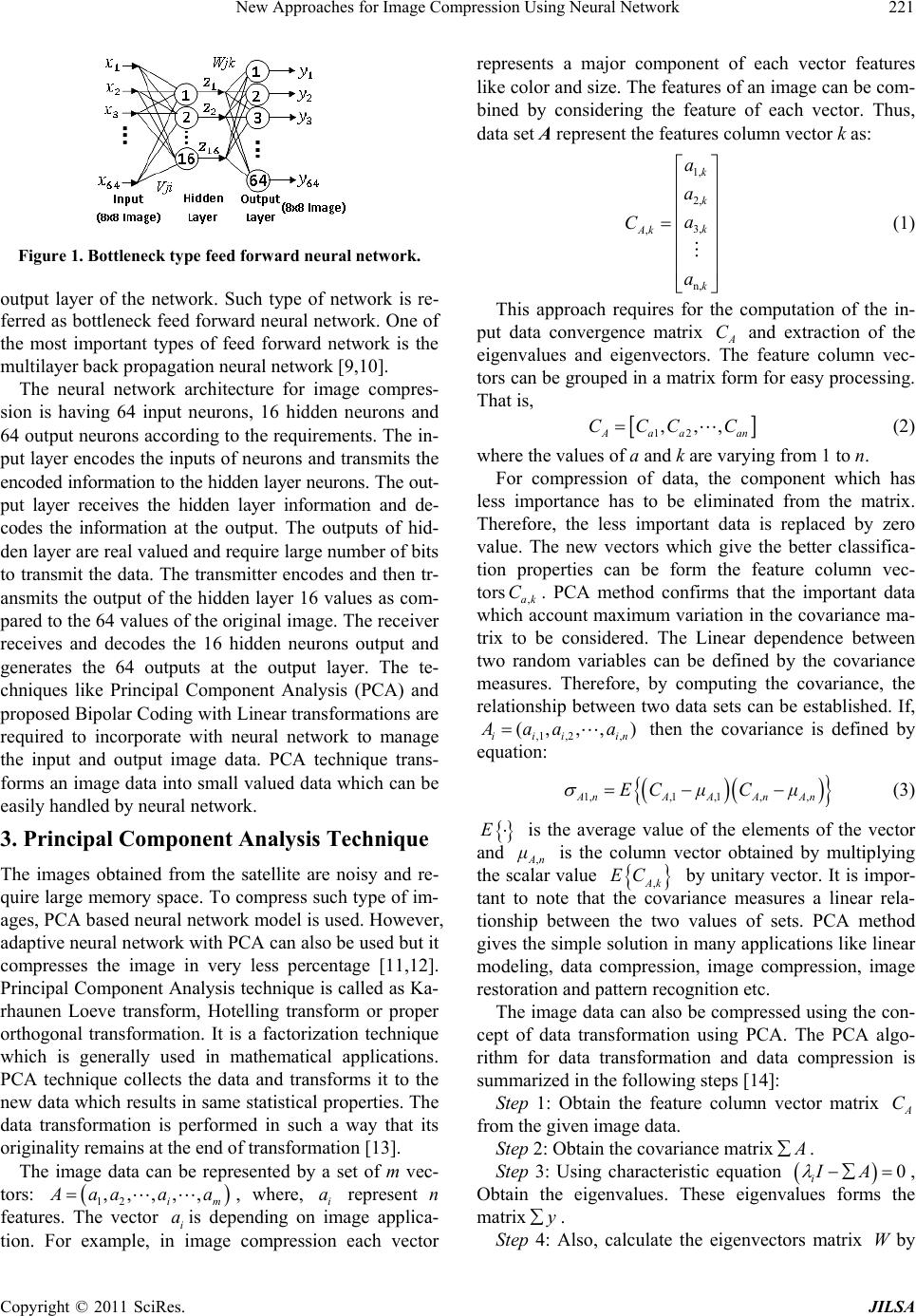 New Approaches for Image Compression Using Neural Network221 Figure 1. Bottleneck type feed forw ard neural networ k. output layer of the network. Such type of network is re- ferred as bottleneck feed forward neural network. One of the most important types of feed forward network is the multilayer back propagation neural network [9,10]. The neural network architecture for image compres- sion is having 64 input neurons, 16 hidden neurons and 64 output neurons according to the requirements. The in- put layer encodes the inputs of neurons and transmits the encoded information to the hidden layer neurons. The out- put layer receives the hidden layer information and de- codes the information at the output. The outputs of hid- den layer are real valued and require large number of bits to transmit the data. The transmitter encodes and then tr- ansmits the output of the hidden layer 16 values as com- pared to the 64 values of the original image. The receiver receives and decodes the 16 hidden neurons output and generates the 64 outputs at the output layer. The te- chniques like Principal Component Analysis (PCA) and proposed Bipolar Coding with Linear transformations are required to incorporate with neural network to manage the input and output image data. PCA technique trans- forms an image data into small valued data which can be easily handled by neural network. 3. Principal Component Analysis Technique The images obtained from the satellite are noisy and re- quire large memory space. To compress such type of im- ages, PCA based neural network model is used. However, adaptive neural network with PCA can also be used but it compresses the image in very less percentage [11,12]. Principal Component Analysis technique is called as Ka- rhaunen Loeve transform, Hotelling transform or proper orthogonal transformation. It is a factorization technique which is generally used in mathematical applications. PCA technique collects the data and transforms it to the new data which results in same statistical properties. The data transformation is performed in such a way that its originality remains at the end of transformation [13]. The image data can be represented by a set of m vec- tors: 12 ,,,,, im aaa a a , where, i represent n features. The vector iis depending on image applica- tion. For example, in image compression each vector represents a major component of each vector features like color and size. The features of an image can be com- bined by considering the feature of each vector. Thus, data set A represent the features column vector k as: a 1, 2, 3, , n, k k k Ak k a a a C a (1) This approach requires for the computation of the in- put data convergence matrix A and extraction of the eigenvalues and eigenvectors. The feature column vec- tors can be grouped in a matrix form for easy processing. That is, C 12 ,,, Aaa an CCC C (2) where the values of a and k are varying from 1 to n. For compression of data, the component which has less importance has to be eliminated from the matrix. Therefore, the less important data is replaced by zero value. The new vectors which give the better classifica- tion properties can be form the feature column vec- tors ,ak. PCA method confirms that the important data which account maximum variation in the covariance ma- trix to be considered. The Linear dependence between two random variables can be defined by the covariance measures. Therefore, by computing the covariance, the relationship between two data sets can be established. If, ,1 C (, ii,2 , ,, ) i in aa a then the covariance is defined by equation: 1,,1 ,1,,A nAAAnAn EC μCμ (3) E is the average value of the elements of the vector and ,An is the column vector obtained by multiplying the scalar value ,Ak EC by unitary vector. It is impor- tant to note that the covariance measures a linear rela- tionship between the two values of sets. PCA method gives the simple solution in many applications like linear modeling, data compression, image compression, image restoration and pattern recognition etc. The image data can also be compressed using the con- cept of data transformation using PCA. The PCA algo- rithm for data transformation and data compression is summarized in the following steps [14]: Step 1: Obtain the feature column vector matrix from the given image data. A C Step 2: Obtain the covariance matrix . Step 3: Using characteristic equation 0 iIA , Obtain the eigenvalues. These eigenvalues forms the matrix y . Step 4: Also, calculate the eigenvectors matrix by W Copyright © 2011 SciRes. JILSA  New Approaches for Image Compression Using Neural Network 222 considering the eigenvaluesi . Step 5: Obtain the Transformation by considering the eigenvectors as their columns. T W Step 6: Obtain the features vector matrix by . T yA CCW Step 7: For compression of an image, the dimensional- ity of the new feature vector is reduce by setting small eigenvalues i to zeros. The dimensionality of input feature vector is changed by considering the small eigenvalues as zeros. The accu- racy of the obtained results depends upon the selected threshold value of an eigenvalue. If the threshold value of eigenvalue is high, then the dimension of feature ei- genvector is reduced more and hence the high compres- sion can be achieved. This method considers only the data which has the maximum variation. Thus, PCA gives the simple solution to achieve high data compression, image compression and eigenface recognition. But, at high threshold eigenvalue, the loss of image data is very large. To overcome this drawback in PCA, authors sug- gested a bottleneck type neural network which is used to change the dimension of feature eigenvector matrix effi- ciently as well as reconstruction of an original image data. The architecture of such bottleneck type feed forward back propagation neural network for compression appli- cation is shown in Figure 1. 4. Training Algorithm for Feed Forward Neural Network To achieve the high compression and faithful decompres- sion of an image, the training algorithm of feed forward back propagation neural network is summarized in the following steps [15]: Step 1: Initially, weights are required to initialize to a small random values. Each input neuron receives the in- put signal xi and transmits to hidden units. Step 2: Hidden units of neural network sums its wei- ghted input signals along with biases as follows: 1` n i inj oji ji zv xv (4) On application of activation function, the output j z and it sends this signal to all neurons of output layer. inj fz k Step 3: Now, output neurons (), add all ,1,, k yk m p weighted inputs, and applies its 1 inkj jk j yw zw ok activation function to calculate the output kin fy k ty Step 4: Output unit compares the calculated output corresponding to a target and error is calculated as, kk ink σfy Step 5: The error from the output is distributed to the hidden layer, then the each hidden unit , sums its inputs from units in the layer , 1,..., j zj n 1 m injj jk kw (6) The error is calculated as, inj inj z (7) Step 6: Each output neuron (k), updates its bias and weights y 1, ,j pand the weights get corrected by kkj wz , similarly the bias corrected by the term Δw ok k . Step 7: The new updated weights are represented by the following terms as; updatedold Δ kjk ww jk w (8) updatedold Δ okok ok www (9) Step 8: The weight correction term for hidden neurons, Δ ijj i vα (10) The bias correction term for hidden neurons, Δ oj j v (11) Step 9: New updated weights are, updatedold Δ ijij ij vvv (12) updatedold Δ ojoj oj vvv (13) Along with PCA algorithm, the above feed forward back propagation algorithm is used to train the neural network. The accuracy of the decompression is depends upon the threshold eigenvalue at which the iteration pro- cess of learning is completed. In PCA technique, it is very difficult to obtain the correct covariance matrix. Similarly, the precise value of eigenvalues and eigenvec- tors is not possible due to computational error and hence the results are not satisfactory. Authors, used the neural network to minimize these errors in PCA, but the decom- pressed results are still not satisfactory. To overcome these problems in PCA, authors proposed another meth- od, Bipolar Coding with linear transformation along with feed forward back propagation neural network. 5. Bipolar Coding Technique The Bipolar Coding technique is a new approach in the field of image processing. The Bipolar Coding transfor- mation is based on the bipolar activation function. The authors have proposed and applied this technique along with neural network for image compression. The sets of data obtained from an image are in analog form and re- quired to convert into digital form. This conversion is po- ssible using bipolar coding with linear scaling. The scal- ing has the advantage of mapping the desired range of (5) Copyright © 2011 SciRes. JILSA  New Approaches for Image Compression Using Neural Network223 maximum and minimum analog value of the data set. The conversions are based on certain ranges where ana- log form is scaled between value 0 and 1. Thus, for con- verting analog values into digital form, different binary values can be assigned. In this technique, each value is converted into the range between 0 and 1 using the for- mula as follows [15]: max min X min Intercept YCXX (14) These converted values are used as the input to the neural network. Even though the neural network archi- tecture takes input from 64 nodes down to 16 nodes, no actual compression has been occurred because unlike the 64 original inputs which are 8-bit pixel values, the out- puts of the hidden layer are also real-valued, which re- quires possibly an infinite number of bits for transmis- sion. True image compression occurs when the hidden layer outputs are digitized before transmission. The Fig- ure 2 shows a typical digitization scheme using 3 bits as reported in [16]. In this scheme, there are 8 possible bi- nary codes: 000, 001, 010, 011, 100, 101, 110, and 111. Each of these codes represents a range of values for a hidden unit output. For example, consider the first hidden output, when the value is between –0.1 and –0.75, then the code 000 is transmitted and when the value is betw- een 0.5 and 0.75, the code 110 is transmitted. The conce- pt of residual blocks conversion also used by G. Qiu et al. [17] but the PSNR observed was very less. The proposed Bipolar Coding technique using feed forward back pro- pagation neural network is summarized in the following steps: Step 1: Divide the image into small 8 × 8 chucks. These chucks are in square matrix form. It is easy to perform operation on such symmetric matrix. Step 2: Obtain the values of pixels (0 to 255) of matrix and convert these values in the bipolar range –1 to 1. This is called as pixel to real number mapping. Step 3: Now apply these values of bipolar range to the feed forward back propagation neural network. This Figure 2. Digitization of hidden unit output. neural network must have 64 input neurons as the chucks are of the size 8 × 8. Train the neural network using training algorithm as explained in Section 4. Step 4: The bipolar values with weight and biases feed to the hidden layer which may have 2, 4, 8, 16, 32, and 64 hidden neurons. Convert these values in digital bits as explain in Section 5. Step 5: Select the 8 × 8 chucks in a sequence after the completion of training of the neural network. Step 6: Digital bits are now converted to real values. Step 7: Matrix ranges bipolar values from –1 to 1 re- converted from real value to (0 to 255) pixel mapping. Step 8: Finally, recall phase demonstrate the decom- pressed image (output image) at the output of the output layer of neural network. Pixel to real value and real value to pixel conversion is done during the compression and decompression process. The proposed Bipolar Coding technique using feed forward back propagation neural network converts deci- mal values into its equivalent binary code and reconvert in decompression phase. The compression and quality of image depends on number of neurons in the hidden layer. The quality of output image improves and the data loss reduces as the number of hidden neurons increases. In PCA technique, the eigenvector matrix obtained from the covariance matrix is consisting of large decimal values. The statistical calculation using these values re- sults in erroneous results. The proposed Bipolar Coding uses the normalized –1 to 1 decimal value and its equi- valent binary bits to represent the image data. The st- atistical calculation in Bipolar Coding becomes less com- plex and therefore the loss of data is reduced. Thus, this technique gives the better result as compared to PCA te- chnique. On other hand, as it is an iterative, it requires large time for data conversion and iterations. It needs lar- ge memory space to store the subsequent results. Some- times, if the image is of more pixel size, then system is unable to perform required number of iterations as it re- quired the more storage space. The output values of the neural network are used for calculation of the updated weights and biases in the next iteration. This problem of neural network learning can be considered as a function of optimization, where network is trying to determine the parameters like weights and biases to minimize the network errors. Authors proposed the use of Levenberg-Marquardt algorithm which acts as optimization technique for fast reduction of an error. Au- thors tried to use these advantages of Levenberg-Mar- quardt in image compression application. The LM algo- rithm overcomes the drawbacks of PCA with neural network and proposed Bipolar Coding technique. 6. Levenberg-Marquardt Algorithm Neural networks are suitable for linear as well as highly Copyright © 2011 SciRes. JILSA 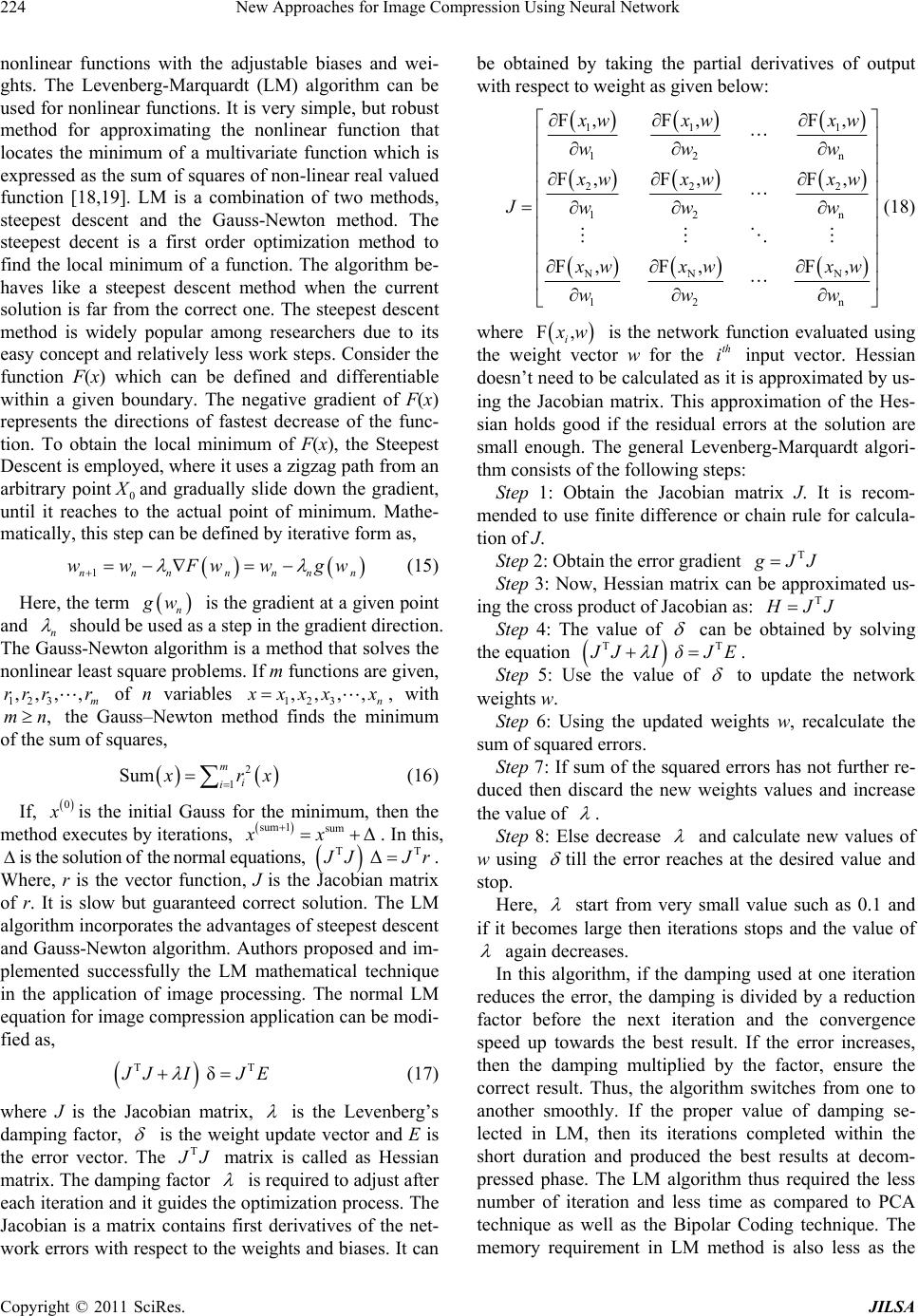 New Approaches for Image Compression Using Neural Network 224 nonlinear functions with the adjustable biases and wei- ghts. The Levenberg-Marquardt (LM) algorithm can be used for nonlinear functions. It is very simple, but robust method for approximating the nonlinear function that locates the minimum of a multivariate function which is expressed as the sum of squares of non-linear real valued function [18,19]. LM is a combination of two methods, steepest descent and the Gauss-Newton method. The steepest decent is a first order optimization method to find the local minimum of a function. The algorithm be- haves like a steepest descent method when the current solution is far from the correct one. The steepest descent method is widely popular among researchers due to its easy concept and relatively less work steps. Consider the function F(x) which can be defined and differentiable within a given boundary. The negative gradient of F(x) represents the directions of fastest decrease of the func- tion. To obtain the local minimum of F(x), the Steepest Descent is employed, where it uses a zigzag path from an arbitrary point0 and gradually slide down the gradient, until it reaches to the actual point of minimum. Mathe- matically, this step can be defined by iterative form as, 1nnn nnn wwFww gw n (15) Here, the term n w is the gradient at a given point and n should be used as a step in the gradient direction. The Gauss-Newton algorithm is a method that solves the nonlinear least square problems. If m functions are given, m of n variables 123 n123 ,,,r,rr r,,,, xx xx, with the Gauss–Newton method finds the minimum of the sum of squares, ,nm 2 1 Sum m i i rx (16) If, 0 is the initial Gauss for the minimum, then the method executes by iterations, . In this, is the solution of the normal equations, sum 1sum Δxx T ΔT JJr. Where, r is the vector function, J is the Jacobian matrix of r. It is slow but guaranteed correct solution. The LM algorithm incorporates the advantages of steepest descent and Gauss-Newton algorithm. Authors proposed and im- plemented successfully the LM mathematical technique in the application of image processing. The normal LM equation for image compression application can be modi- fied as, T δT JI JE (17) where J is the Jacobian matrix, is the Levenberg’s damping factor, is the weight update vector and E is the error vector. The T J matrix is called as Hessian matrix. The damping factor is required to adjust after each iteration and it guides the optimization process. The Jacobian is a matrix contains first derivatives of the net- work errors with respect to the weights and biases. It can be obtained by taking the partial derivatives of output with respect to weight as given below: 11 1 12 22 2 12 NN N 12 F, F,F, F, F,F, F, F,F, n n n wxw xw ww w wxw xw Jww w wxw xw ww w (18) where F, i w is the network function evaluated using the weight vector w for the input vector. Hessian doesn’t need to be calculated as it is approximated by us- ing the Jacobian matrix. This approximation of the Hes- sian holds good if the residual errors at the solution are small enough. The general Levenberg-Marquardt algori- thm consists of the following steps: th i Step 1: Obtain the Jacobian matrix J. It is recom- mended to use finite difference or chain rule for calcula- tion of J. Step 2: Obtain the error gradient T JJ Step 3: Now, Hessian matrix can be approximated us- ing the cross product of Jacobian as: T JJ Step 4: The value of can be obtained by solving the equation TT JJ I δ E . Step 5: Use the value of to update the network weights w. Step 6: Using the updated weights w, recalculate the sum of squared errors. Step 7: If sum of the squared errors has not further re- duced then discard the new weights values and increase the value of . Step 8: Else decrease and calculate new values of w using till the error reaches at the desired value and stop. Here, start from very small value such as 0.1 and if it becomes large then iterations stops and the value of again decreases. In this algorithm, if the damping used at one iteration reduces the error, the damping is divided by a reduction factor before the next iteration and the convergence speed up towards the best result. If the error increases, then the damping multiplied by the factor, ensure the correct result. Thus, the algorithm switches from one to another smoothly. If the proper value of damping se- lected in LM, then its iterations completed within the short duration and produced the best results at decom- pressed phase. The LM algorithm thus required the less number of iteration and less time as compared to PCA technique as well as the Bipolar Coding technique. The memory requirement in LM method is also less as the Copyright © 2011 SciRes. JILSA 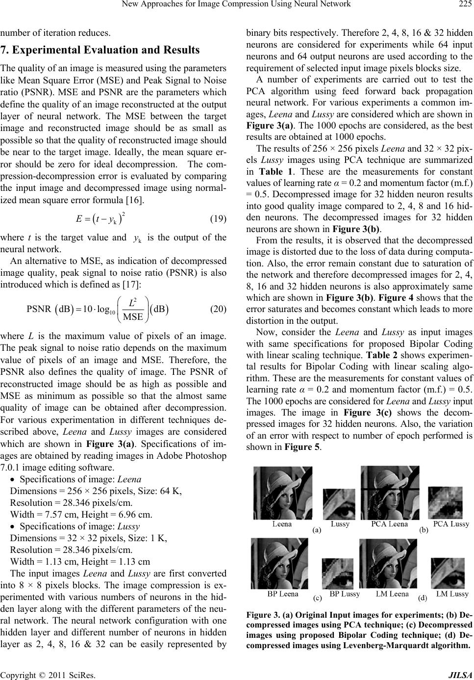 New Approaches for Image Compression Using Neural Network225 number of iteration reduces. 7. Experimental Evaluation and Results The quality of an image is measured using the parameters like Mean Square Error (MSE) and Peak Signal to Noise ratio (PSNR). MSE and PSNR are the parameters which define the quality of an image reconstructed at the output layer of neural network. The MSE between the target image and reconstructed image should be as small as possible so that the quality of reconstructed image should be near to the target image. Ideally, the mean square er- ror should be zero for ideal decompression. The com- pression-decompression error is evaluated by comparing the input image and decompressed image using normal- ized mean square error formula [16]. 2 k Ety (19) where t is the target value and is the output of the neural network. k y An alternative to MSE, as indication of decompressed image quality, peak signal to noise ratio (PSNR) is also introduced which is defined as [17]: 2 10 PSNR dB10logdB MSE L (20) where L is the maximum value of pixels of an image. The peak signal to noise ratio depends on the maximum value of pixels of an image and MSE. Therefore, the PSNR also defines the quality of image. The PSNR of reconstructed image should be as high as possible and MSE as minimum as possible so that the almost same quality of image can be obtained after decompression. For various experimentation in different techniques de- scribed above, Leena and Lussy images are considered which are shown in Figure 3(a). Specifications of im- ages are obtained by reading images in Adobe Photoshop 7.0.1 image editing software. Specifications of image: Leena Dimensions = 256 × 256 pixels, Size: 64 K, Resolution = 28.346 pixels/cm. Width = 7.57 cm, Height = 6.96 cm. Specifications of image: Lussy Dimensions = 32 × 32 pixels, Size: 1 K, Resolution = 28.346 pixels/cm. Width = 1.13 cm, Height = 1.13 cm The input images Leena and Lussy are first converted into 8 × 8 pixels blocks. The image compression is ex- perimented with various numbers of neurons in the hid- den layer along with the different parameters of the neu- ral network. The neural network configuration with one hidden layer and different number of neurons in hidden layer as 2, 4, 8, 16 & 32 can be easily represented by binary bits respectively. Therefore 2, 4, 8, 16 & 32 hidden neurons are considered for experiments while 64 input neurons and 64 output neurons are used according to the requirement of selected input image pixels blocks size. A number of experiments are carried out to test the PCA algorithm using feed forward back propagation neural network. For various experiments a common im- ages, Leena and Lussy are considered which are shown in Figure 3(a). The 1000 epochs are considered, as the best results are obtained at 1000 epochs. The results of 256 × 256 pixels Leena and 32 × 32 pix- els Lussy images using PCA technique are summarized in Table 1. These are the measurements for constant values of learning rate α = 0.2 and momentum factor (m.f.) = 0.5. Decompressed image for 32 hidden neuron results into good quality image compared to 2, 4, 8 and 16 hid- den neurons. The decompressed images for 32 hidden neurons are shown in Fi gure 3(b). From the results, it is observed that the decompressed image is distorted due to the loss of data during computa- tion. Also, the error remain constant due to saturation of the network and therefore decompressed images for 2, 4, 8, 16 and 32 hidden neurons is also approximately same which are shown in Figure 3(b). Figure 4 shows that the error saturates and becomes constant which leads to more distortion in the output. Now, consider the Leena and Lussy as input images with same specifications for proposed Bipolar Coding with linear scaling technique. Table 2 shows experimen- tal results for Bipolar Coding with linear scaling algo- rithm. These are the measurements for constant values of learning rate α = 0.2 and momentum factor (m.f.) = 0.5. The 1000 epochs are considered for Leena and Lussy input images. The image in Figure 3(c) shows the decom- pressed images for 32 hidden neurons. Also, the variation of an error with respect to number of epoch performed is shown in Figure 5. Figure 3. (a) Original Input images for experiments; (b) De- compressed images using PCA tec hnique; (c) Decompressed images using proposed Bipolar Coding technique; (d) De- compressed images using Levenberg-Marquardt algorithm. Copyright © 2011 SciRes. JILSA 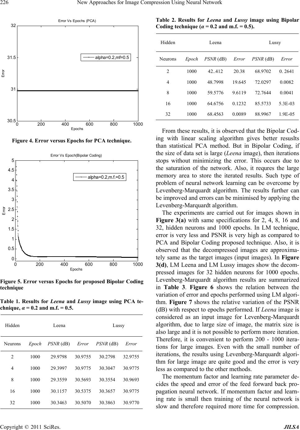 New Approaches for Image Compression Using Neural Network 226 0200 400 600 8001000 30.5 31 31.5 32 E poc hs E rror E rror V s Ep ochs (P CA ) alpha=0.2,mf=0.5 Figure 4. Error versus Epochs for PCA technique. 0200 400600800 1000 0 0.5 1 1.5 2 2.5 3 3.5 4 4.5 5 E poc hs Error E rror V s Epoch(Bi pol ar Codi ng) alpha=0.2,m.f.=0.5 Figure 5. Error versus Epochs for proposed Bipolar Coding technique Table 1. Results for Leena and Lussy image using PCA te- chnique, α = 0.2 a nd m.f. = 0.5. Hidden Leena Lussy Neurons Epoch PSNR (dB) Error PSNR (dB) Error 2 1000 29.9798 30.9755 30.2798 32.9755 4 1000 29.3997 30.9775 30.3047 30.9775 8 1000 29.3559 30.5693 30.3554 30.9693 16 1000 30.1157 30.5375 30.3657 30.9775 32 1000 30.3463 30.5070 30.3863 30.9770 Table 2. Results for Leena and Lussy image using Bipolar Coding technique (α = 0.2 and m.f. = 0.5). HiddenLeena Lussy Neurons Epoch PSNR (dB) Error PSNR (dB) Error 2 1000 42..41220.38 68.97020. 2641 4 1000 48.799819.645 72.02970.0082 8 1000 59.57769.6119 72.76440.0041 16 1000 64.67560.1232 85.57335.3E-03 32 1000 68.45630.0089 88.99671.9E-05 From these results, it is observed that the Bipolar Cod- ing with linear scaling algorithm gives better resuslts than statistical PCA method. But in Bipolar Coding, if the size of data set is large (Leena image), then iterations stops without minimizing the error. This occurs due to the saturation of the network. Also, it requres the large memory area to store the iterated results. Such type of problem of neural network learning can be overcome by Levenberg-Marquardt algorithm. The results further can be improved and errors can be minimised by applying the Levenberg-Marquardt algorithm. The experiments are carried out for images shown in Figure 3(a) with same specifications for 2, 4, 8, 16 and 32, hidden neurons and 1000 epochs. In LM technique, error is very less and PSNR is very high as compared to PCA and Bipolar Coding proposed technique. Also, it is observed that the decompressed images are approxima- tely same as the target images (input images). In Figure 3(d), LM Leena and LM Lussy images show the decom- pressed images for 32 hidden neurons for 1000 epochs. Levenberg-Marquardt algorithm results are summarized in Table 3. Figure 6 shows the relation between the variation of error and epochs performed using LM algori- thm. Figure 7 shows the relative variation of the PSNR (dB) with respect to epochs performed. If Leena image is considered as an input image for Levenberg-Marquardt algorithm, due to large size of image, the matrix size is also large and it is not possible to perform more iteration. Therefore, it is convenient to perform 200 - 1000 itera- tions for large images. Even with the small number of iterations, the results using Levenberg-Marquardt algori- thm for large image are quite good and the error is very less as compared to the other methods. The momentum factor and learning rate parameter de- cides the speed and error of the feed forward back pro- pagation neural network. If momentum factor and learn- ing rate is small then training of the neural network is slow and therefore required more time for compression. Copyright © 2011 SciRes. JILSA 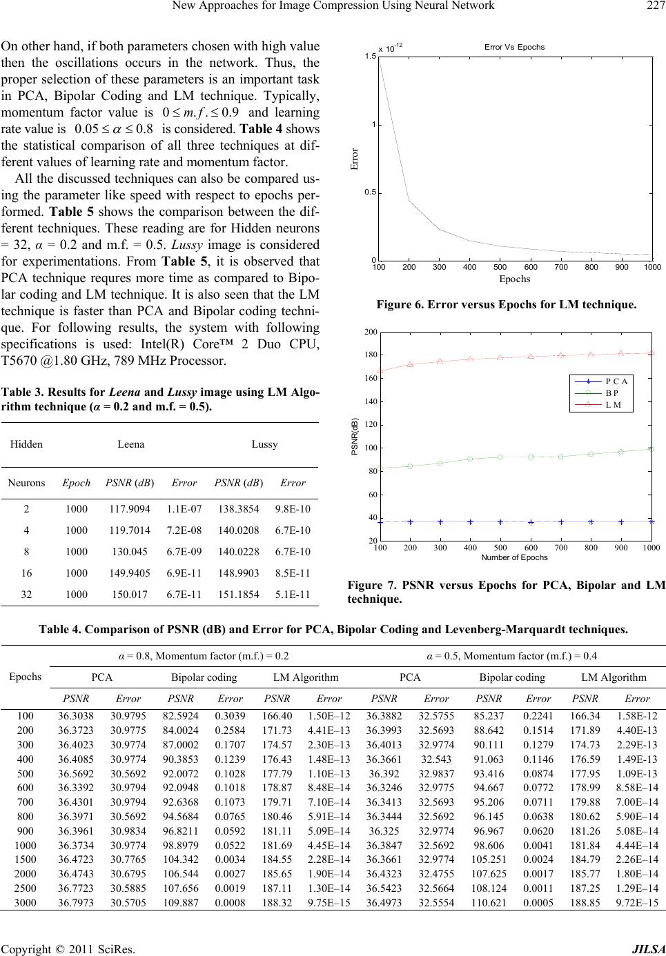 New Approaches for Image Compression Using Neural Network Copyright © 2011 SciRes. JILSA 227 9 On other hand, if both parameters chosen with high value then the oscillations occurs in the network. Thus, the proper selection of these parameters is an important task in PCA, Bipolar Coding and LM technique. Typically, momentum factor value is 0..0.mf and learning rate value is 0.05 0.8 is considered. Ta ble 4 shows the statistical comparison of all three techniques at dif- ferent values of learning rate and momentum factor. 100 200 300 400 500 600 700 800 9001000 0 0. 5 1 1.5 x 10 -12 Epochs Error E rror V s Ep ochs All the discussed techniques can also be compared us- ing the parameter like speed with respect to epochs per- formed. Table 5 shows the comparison between the dif- ferent techniques. These reading are for Hidden neurons = 32, α = 0.2 and m.f. = 0.5. Lussy image is considered for experimentations. From Table 5, it is observed that PCA technique requres more time as compared to Bipo- lar coding and LM technique. It is also seen that the LM technique is faster than PCA and Bipolar coding techni- que. For following results, the system with following specifications is used: Intel(R) Core™ 2 Duo CPU, T5670 @1.80 GHz, 789 MHz Processor. Figure 6. Error versus Epochs for LM technique. Table 3. Results for Leena and Lussy image using LM Algo- rithm technique (α = 0.2 and m.f. = 0.5). Hidden Leena Lussy Neurons Epoch PSNR (dB) Error PSNR (dB)Error 2 1000 117.9094 1.1E-07 138.3854 9.8E-10 4 1000 119.7014 7.2E-08 140.0208 6.7E-10 8 1000 130.045 6.7E-09 140.0228 6.7E-10 16 1000 149.9405 6.9E-11 148.9903 8.5E-11 32 1000 150.017 6.7E-11 151.1854 5.1E-11 100 200300400 500 600 700 800 9001000 20 40 60 80 100 120 140 160 180 200 Number of Epochs PSNR(dB) P C A B P L M Figure 7. PSNR versus Epochs for PCA, Bipolar and LM technique. Table 4. Comparison of PSNR (dB) and Error for PCA, Bipolar Coding and Levenberg-Marquardt technique s. α = 0.8, Momentum factor (m.f.) = 0.2 α = 0.5, Momentum factor (m.f.) = 0.4 PCA Bipolar coding LM Algorithm PCA Bipolar coding LM Algorithm Epochs PSNR Error PSNR Error PSNR Error PSNR Error PSNR Error PSNR Error 100 36.3038 30.9795 82.5924 0.3039 166.401.50E–1236.3882 32.575585.237 0.2241 166.34 1.58E-12 200 36.3723 30.9775 84.0024 0.2584 171.734.41E–1336.3993 32.569388.642 0.1514 171.89 4.40E-13 300 36.4023 30.9774 87.0002 0.1707 174.572.30E–1336.4013 32.977490.111 0.1279 174.73 2.29E-13 400 36.4085 30.9774 90.3853 0.1239 176.431.48E–1336.366132.543 91.063 0.1146 176.59 1.49E-13 500 36.5692 30.5692 92.0072 0.1028 177.791.10E–1336.392 32.983793.416 0.0874 177.95 1.09E-13 600 36.3392 30.9794 92.0948 0.1018 178.878.48E–1436.3246 32.977594.667 0.0772 178.99 8.58E–14 700 36.4301 30.9794 92.6368 0.1073 179.717.10E–1436.3413 32.569395.206 0.0711 179.88 7.00E–14 800 36.3971 30.5692 94.5684 0.0765 180.465.91E–1436.3444 32.569296.145 0.0638 180.62 5.90E–14 900 36.3961 30.9834 96.8211 0.0592 181.115.09E–1436.325 32.977496.967 0.0620 181.26 5.08E–14 1000 36.3734 30.9774 98.8979 0.0522 181.694.45E–1436.3847 32.569298.606 0.0041 181.84 4.44E–14 1500 36.4723 30.7765 104.342 0.0034 184.552.28E–1436.3661 32.9774 105.251 0.0024 184.79 2.26E–14 2000 36.4743 30.6795 106.544 0.0027 185.651.90E–1436.4323 32.4755 107.625 0.0017 185.77 1.80E–14 2500 36.7723 30.5885 107.656 0.0019 187.111.30E–1436.5423 32.5664 108.124 0.0011 187.25 1.29E–14 3000 36.7973 30.5705 109.887 0.0008 188.329.75E–1536.4973 32.5554 110.621 0.0005 188.85 9.72E–15 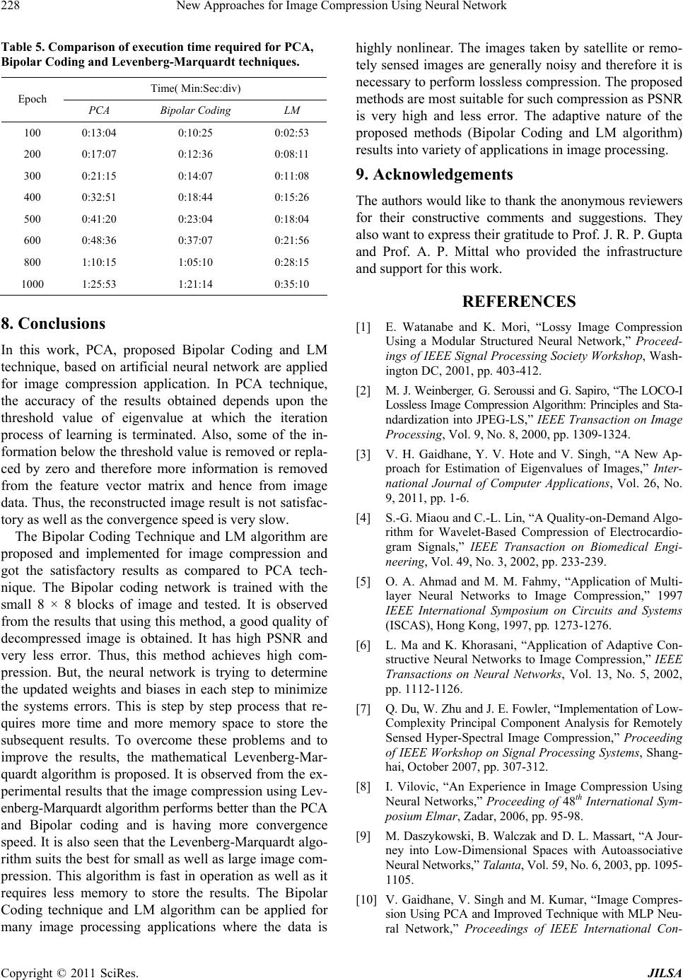 New Approaches for Image Compression Using Neural Network 228 Table 5. Comparison of execution time required for PCA, Bipolar Coding and Levenberg-Marquardt technique s. Time( Min:Sec:div) Epoch PCA Bipolar Coding LM 100 0:13:04 0:10:25 0:02:53 200 0:17:07 0:12:36 0:08:11 300 0:21:15 0:14:07 0:11:08 400 0:32:51 0:18:44 0:15:26 500 0:41:20 0:23:04 0:18:04 600 0:48:36 0:37:07 0:21:56 800 1:10:15 1:05:10 0:28:15 1000 1:25:53 1:21:14 0:35:10 8. Conclusions In this work, PCA, proposed Bipolar Coding and LM technique, based on artificial neural network are applied for image compression application. In PCA technique, the accuracy of the results obtained depends upon the threshold value of eigenvalue at which the iteration process of learning is terminated. Also, some of the in- formation below the threshold value is removed or repla- ced by zero and therefore more information is removed from the feature vector matrix and hence from image data. Thus, the reconstructed image result is not satisfac- tory as well as the convergence speed is very slow. The Bipolar Coding Technique and LM algorithm are proposed and implemented for image compression and got the satisfactory results as compared to PCA tech- nique. The Bipolar coding network is trained with the small 8 × 8 blocks of image and tested. It is observed from the results that using this method, a good quality of decompressed image is obtained. It has high PSNR and very less error. Thus, this method achieves high com- pression. But, the neural network is trying to determine the updated weights and biases in each step to minimize the systems errors. This is step by step process that re- quires more time and more memory space to store the subsequent results. To overcome these problems and to improve the results, the mathematical Levenberg-Mar- quardt algorithm is proposed. It is observed from the ex- perimental results that the image compression using Lev- enberg-Marquardt algorithm performs better than the PCA and Bipolar coding and is having more convergence speed. It is also seen that the Levenberg-Marquardt algo- rithm suits the best for small as well as large image com- pression. This algorithm is fast in operation as well as it requires less memory to store the results. The Bipolar Coding technique and LM algorithm can be applied for many image processing applications where the data is highly nonlinear. The images taken by satellite or remo- tely sensed images are generally noisy and therefore it is necessary to perform lossless compression. The proposed methods are most suitable for such compression as PSNR is very high and less error. The adaptive nature of the proposed methods (Bipolar Coding and LM algorithm) results into variety of applications in image processing. 9. Acknowledgements The authors would like to thank the anonymous reviewers for their constructive comments and suggestions. They also want to express their gratitude to Prof. J. R. P. Gupta and Prof. A. P. Mittal who provided the infrastructure and support for this work. REFERENCES [1] E. Watanabe and K. Mori, “Lossy Image Compression Using a Modular Structured Neural Network,” Proceed- ings of IEEE Signal Processing Society Workshop, Wash- ington DC, 2001, pp. 403-412. [2] M. J. Weinberger, G. Seroussi and G. Sapiro, “The LOCO-I Lossless Image Compression Algorithm: Principles and Sta- ndardization into JPEG-LS,” IEEE Transaction on Image Processing, Vol. 9, No. 8, 2000, pp. 1309-1324. [3] V. H. Gaidhane, Y. V. Hote and V. Singh, “A New Ap- proach for Estimation of Eigenvalues of Images,” Inter- national Journal of Computer Applications, Vol. 26, No. 9, 2011, pp. 1-6. [4] S.-G. Miaou and C.-L. Lin, “A Quality-on-Demand Algo- rithm for Wavelet-Based Compression of Electrocardio- gram Signals,” IEEE Transaction on Biomedical Engi- neering, Vol. 49, No. 3, 2002, pp. 233-239. [5] O. A. Ahmad and M. M. Fahmy, “Application of Multi- layer Neural Networks to Image Compression,” 1997 IEEE International Symposium on Circuits and Systems (ISCAS), Hong Kong, 1997, pp. 1273-1276. [6] L. Ma and K. Khorasani, “Application of Adaptive Con- structive Neural Networks to Image Compression,” IEEE Transactions on Neural Networks, Vol. 13, No. 5, 2002, pp. 1112-1126. [7] Q. Du, W. Zhu and J. E. Fowler, “Implementation of Low- Complexity Principal Component Analysis for Remotely Sensed Hyper-Spectral Image Compression,” Proceeding of IEEE Workshop on Signal Processing Systems, Shang- hai, October 2007, pp. 307-312. [8] I. Vilovic, “An Experience in Image Compression Using Neural Networks,” Proceeding of 48th International Sym- posium Elmar, Zadar, 2006, pp. 95-98. [9] M. Daszykowski, B. Walczak and D. L. Massart, “A Jour- ney into Low-Dimensional Spaces with Autoassociative Neural Networks,” Talanta, Vol. 59, No. 6, 2003, pp. 1095- 1105. [10] V. Gaidhane, V. Singh and M. Kumar, “Image Compres- sion Using PCA and Improved Technique with MLP Neu- ral Network,” Proceedings of IEEE International Con- Copyright © 2011 SciRes. JILSA  New Approaches for Image Compression Using Neural Network229 ference on Advances in Recent Technologies in Commu- nication and Computing, Kottayam, 16-17 October 2010, pp. 106-110. [11] R. C. Gonzalez, R. E. Woods and S. L. Eddins, “Digital Image Processing Using MATLAB,” Pearson Edition, Dorling Kindersley, London, 2003. [12] J.-X. Mi and D.-S. Huang, “Image Compression Using Principal Component Analysis Neural Network,” 8th IEEE International Conference on Control, Automation, Robotics and Vision, Kunming, 6-9 December 2004, pp. 698-701. [13] S.-T. Bow, B. T. Bow and S. T. Bow, “Pattern Recogni- tion and Image Processing,” Revised and Expanded, 2nd Edition, CRC Press, Boca Raton, 2002. [14] M. Nixon and A. Aguado, “Feature Extraction & Image Processing,” 2nd Edition, Academic Press, Cambridge, 2008, pp. 385-398. [15] S. N. Sivanandam, S. Sumathi and S. N. Deepa, “Introdu- ction to Neural Network Using MATLAB 6.0,” 2nd Edi- tion, Tata Mc-Graw Hill Publication, Boston, 2008. [16] A. Laha, N. R. Pal and B. Chanda, “Design of Vector Quantizer for Image Compression Using Self Organizing Feature Map and Surface Fitting,” IEEE Transactions on Image Processing, Vol. 13, No. 10, October 2004, pp. 1291-1303. doi:10.1109/TIP.2004.833107 [17] G. Qiu, T. J. Terrell and M. R. Varley, “Improved Image Compression Using Back Propagation Networks,” In: P. J. G. Lisbao and M. J. Taylor, Eds., Proceeding of the Workshop on Neural Network Applications and Tools, IEEE Computer Society Press, Washington DC, 1994, pp. 73-81. [18] V. Singh, I. Gupta and H. O. Gupta, “ANN Based Esti- mator for Distillation Using Levenberg-Marquardt Ap- proach,” Engineering Applications of Artificial Intelli- gence, Vol. 20, No. 2, 2007, pp. 249-259. doi:10.1016/j.engappai.2006.06.017 [19] M. I. A. Lourakis, “A Brief Description of the Levenberg- Marquardt Algorithm Implemented by Levmar,” Founda- tion of Research and Technology, Vol. 4, 2005, pp. 1-6. Copyright © 2011 SciRes. JILSA
|