Journal of Intelligent Learning Systems and Applications, 2011, 3, 209-219
doi:10.4236/jilsa.2011.34024 Published Online November 2011 (http://www.SciRP.org/journal/jilsa)
209
Chinese Stock Price and Volatility Predictions with
Multiple Technical Indicators
Qin Qin, Qing-Guo Wang, Shuzhi Sam Ge, Ganesh Ramakrishnan
Department of Electrical and Computer Engineering, National University of Singapore, Singapore City, Singapore.
Received July 19th, 2011; revised September 19th, 2011; accepted October 8th, 2011.
ABSTRACT
While a large number o f studies have been reported in the literatu re with reference to the use o f Regression model and
Artificial Neural Network (ANN) models in predicting stock prices in western countries, the Chinese stock market is
much less studied. Note that the latter is growing rapidly, will overtake USA one in 20 - 30 years time and thus becomes
a very important place for investors worldwide. In this paper, an attemp t is made at pred icting th e Shanghai Compo site
Index returns and price volatility, on a daily and weekly basis. In the paper, two different types of prediction models,
namely the Regression and Neural Network models are used for the prediction task and multiple technical indicators
are included in the models as inputs. The performances of the two models are compared and evaluated in terms of di-
rectional accuracy. Their performances are also rigorously compared in terms of economic criteria like annualized
return rate (ARR) from simulated trading. In this paper, both trading with and without short selling has been consid-
ered, and the results show in most cases, trading with short selling leads to higher p rofits. Also, both the ca ses with and
without commission costs are discussed to show the effects of commission costs when the trading systems are in actual
use.
Keywords: Regression Model, Artificial Neural Network Model, Chinese Stock Market, Technical In di cators, Volatility
1. Introduction
From the beginning of time it has been man’s common
goal to make his life easier. The prevailing notion in so-
ciety is that wealth brings comfort an d luxury, so it is not
surprising that there has been so much work done on
ways to predict the markets. Various technical, funda-
mental, and statistical indicators have been proposed and
used with varying results. However, no one technique or
combination of techniques has been successful enough to
consistently “beat the market”. As a result, there is a hu-
ge motivation to develop new forecasting techniques that
can unravel the market’s mysteries and obtain greater pr-
ofits.
The stock market is known as the “cradle of capital-
ism”. It is a place where companies come to raise their
share capital and investors go to invest their surplus fun-
ds. Vast amounts of capital are invested and traded in ev-
eryday all over the world. The prediction of the stock
market movements, however, poses a challenge to aca-
demicians and practitioners. The reason is that stock mar-
ket movements are characterized as being uncertain and
complex as it can be affected by virtually any economic,
social or political development that has a bearing on the
economy. This uncertainty and complexity i s undesirable
for any trader who is attempting to make prof its from the
stock market. Therefore, there is a need to reduce this
uncertainty by making accurate predictions.
Initially, stock market research encapsulated two ele-
mental trading techniques namely the Technical and Fun-
damental approaches [1]. In Technical analysis, it is beli-
eved that market timing is keypoint. It involves the study
of historical data of the stock market to predict trends in
price and volume. In other words, there is heavy reliance
on historical data in order to predict future outcomes.
Fundamental analysis, on the other hand involves making
estimates on the intrinsic value of a stock. This techn ique
uses information such as earnings, ratios, and manage-
ment effectiveness to predict future outcomes.
As the level of investing and trading grew, there began
a pursuit for better tools and methods that could not only
increase gains but also minimize the risks undertaken by
the investor. Tools that used modeling techniques to dis-
cover patterns within the historical data of the stock mar-
ket were put to test, with an attempt to p redict and bene-

Chinese Stock Price and Volatility Predictions with Multiple Technical Indicators
210
fit from the market’s direction. One such example is the
Linear Time Series Models, where univariate and multi-
variate regression models [2] were used to identify pat-
terns in the historical data of the stock market. For non-
linear patterns, Machine Learning Models [3], in parti-
cular neural networks, were commonly used. For exam-
ple, one sees that:
 In [4], the authors used a mean reverting charac-
teristic to model and estimate the stock markets.
The authors stated that the random walk which is
used to describe the stock markets may not be cor-
rect when the process of stock markets diverge
over time. The mean reverting characteristic is a
good way to model and estimate the stock mark ets.
The authors used two methods to estimate the pa-
rameters, which are Least Square Estimation and
Maximum Likelihood Estimation. In this paper,
the authors focused on the monthly data of Dow
Jones Industrial Average and the Singapore Straits
Times Index and got some interesting conclusion.
 In [5], the authors predicted the mid-term price
trend for Taiwan stock market. The authors firstly
extracted the features from ARIMA analyses, then
the authors used the features which are produced
in the first step to train a recurrent neural network.
The Taiwan stock market series is regarded by the
authors as a nonlinear ARIMA (1,2,1). The concl-
usion of this paper is that the prediction system
can predict the Taiwan sto ck market trend of up to
6 weeks based on four years weekly data with an
acceptable accuracy.
 In [6], the authors focused the research work on
Shanghai stock market for Chinese stock market
is one of fast growing stock markets in the world.
The authors used two types of models which are
the model of stochastic SARIMA and the model
of backpropagation network. The author used the
actual data of Shanghai Composite Index to do the
prediction and found that SARIMA model is more
optimistic.
 In [7], the autho rs took advantage of the nonlinear
dynamical theory to use the multivariate nonlin ear
prediction method. The prediction system is based
on the reconstruction of multidimensional phase
space. The authors set the model using multivari-
ate nonlinear prediction method and got the expe-
riment results using the data of Shenzhen Index.
The authors compared the results obtained using
multivariate nonlinear prediction method with the
results obtained using unvariate nonlinear predic-
tion method and found that the performance of
multivariate nonlinear prediction method is better
than the performance of unvariate nonlinear pre-
diction method.
 In [8], the author stated that the stock market is a
very complicated nonlinear system, the artificial
neural network also has nonlinear characteristic. It
is proper to use artificial neural network to do the
prediction of stock market. The authors used the
artificial neural network to imitate the trading pro-
cess of stock market. Because the convergent spe-
ed of backpropagation algorithm is low, the auth-
ors enhanced the convergent speed of backpropa-
gation algorithm by proposing the rate of devia-
tion. The authors used the data of both Shanghai
and Shenzhen to do the prediction.
 In [9], the authors explored a new method to esti-
mate the systematic risk (which is called as beta)
in China stock market. A technique is involved in
this new method, which is maximal overlap discr-
ete wavelet transform (MODWT). The technique
will not lose any in formation when it is investiga-
ting the behavior of beta at different time frames.
The experimental results showed that China stock
market is quite different from other stock markets.
The authors drew a conclusion that the difference
between China stock market and other stock mar-
kets is due to the character and behavior finance.
 In [10], the authors analyzed the volatility of a
stock in China on its returns series using th e mod-
els of GARCH family. They found that the series
of stock returns is st at i onary , and i t has a si gni fi cant
ARCH effect, a volatility cluster exists in China
stock market. The authors also found that a return
of negative shock produces more volatility than
the positive one of equal magnitude. They finally
drew a conclusion that there is a leverage effect in
stock returns volatility.
 In [11], the authors used the daily data of Shang-
hai stocks to do the prediction based on the family
GARCH models. The paper used ME, MAE and R-
MSE for error measurement. From the results, the
authors found that in the training period, EGAR-
CH-M model can generate best performance, whi-
le in testing period, simple GARCH model or asy-
mmetric model can produce best performance.
In general, most of stock market studies in the litera-
ture have been focused on developed markets while em-
erging markets are much less studied. Note that the latter
is growing rapidly, and in particular, China market will
overtake USA one in 20 - 30 years time and it has beco-
mes a very important place for investors worldwide. It is
thus timely to study this market's performance and effi-
ciency based on recent data. This paper attempts to predi-
ct the Shanghai Co mposite Index return and volatility on
a daily and weekly basis with use of multiple technical

Chinese Stock Price and Volatility Predictions with Multiple Technical Indicators211
indicators. Specifically, the present work contributes to
the literature in the following ways:
1) An attempt is made to understand the efficacy of an
emerging market such as China. Today, China is one of
the fastest growing emerging economies in the world. Not
only is there a significant growth in the demand for invest-
ment funds but the growth in capital markets is also ex-
pected to play an increasingly important role in the pro c-
ess. At this transitional stage, it is necessary to assess the
level of efficiency of the Chinese Stock Market in order
to establish its longer term role in the process of econo-
mic development. However as studies on Chinese Stock
Markets are very few and also dated and mostly inconcl-
usive, the objective of this study in this paper is to test
whether predictability of return rates and price volatility
is possible.
2) An attempt is made to predict stock market price
volatility. Volatility is an important indicator for inves-
tors. Results from this study do show that neural network
models have their merits and perform better than regres-
sion models.
3) Multiple technical indicators are used in modeling.
We also use different combinations of different technical
indicators to do the prediction to see the performance.
Some combinations improve the performance of the pre-
diction.
The rest of the paper is organized as follows. Section 2
gives an overview of the stock market prediction meth-
ods. Section 3 presents the methodology and shows the
results for the predictability of Shanghai Composite In-
dex return. Section 4 presents the methodology and sho-
ws the results for the predictability of Shanghai Compos-
ite Index price volatility. Finally, Section 5 gives a con-
clusion of the work that has been done, as well as possi-
ble areas of improvements in future work.
2. Stock Market Prediction Methods
In this section, we will consider the different prediction
methods that are available for predicting stock market
movements and returns. Some o f these methods that will
be covered in depth in this section are Technical Analysis,
Linear Time Series Models and Machine Learning Mod-
els.
2.1. Technical Analysis
The idea behind technical analysis is that stock prices
move in trends dictated by the constan tly changing attitu-
des of investors in response to different forces. Future
stock movements are predicted by using price, volume
and observing trends that are dominating the market. Te-
chnical analysis rests on the assumption that history re-
peats itself and that future market direction can be deter-
mined by examining past prices [1]. The groups of pro-
fessionals who subscribe to this method are the technical
analysts or the chartists, as they are more commonly kn-
own. To them all information about earnings, dividends
and future performance of the company is already refl-
ected in the stock’s price history. Therefore the historical
price chart is all a chartist needs to make predictions of
future stoc k price movem e nt s .
This method of predicting the market is highly critici-
zed because it is highly subjective. Two technical analy-
sts studying the same chart may interpret them different-
ly, thereby arriving at completely differen t trading strate-
gies. Also a chartist may only occasionally be successful
if trends perpetuate. Technical analysis is also considered
to be controversial as it contradicts the Efficient Market
Hypothesis. Despite such criticism and controversy, the
method of technical analysis is used by approximately
90% of the major stock traders.
In this paper, several technical indicators are used. I
will show the details of the technical indicators blow:
1) Moving Average: This indicator returns the mov-
ing average of a field over a given period of time. This is
done primarily to avoid noise in the daily price move-
ments. The formula of MA used in this chapter is showed
below:
mean (last n close prices)
n
MA

(1)
The n is the parameter. We set n as 10 and 25 in this pa-
per.
2) Oscillator: This function compares a security’s
closing price to its price range over a given time period.
The formula of SO used in this chapter is showed below:
close price
%100 n
nn
L
KHL

  (2)
%3period moving average of %DK

 (3)
where n
H
and n are respectively the highest and the
lowest price over the last n periods. The n is the parame-
ter. We set n as 10.
L
3) Volatility: Vo latility can either be measured by us-
ing the standard deviation or variance between returns
from the stock or market index. Commonly, the higher
the volatility, the riskier th e stock or market. The formula
of volatility used in th is chapter is showed below:


Volatility = stdlast close pricesn (4)
The n is the parameter. We set n as 10.
Beside the technical indicators above, we also used
some simple technical indicators: return, actual price
change, volume and volume difference.
2.2. Linear Time Series Models
Linear time series models are often us ed to predict future
values of the time series by detecting linear relationships

Chinese Stock Price and Volatility Predictions with Multiple Technical Indicators
212
between the historical data of the stock and the time se-
ries under consider ation. [2 ] De pending on th e nu mber of
different variables used as factors of the time series, two
different types of linear time series models are used. For
the case where only one factor is used to predict th e time
series, univariate regression is employed. If more vari-
ables are used to predict the time series, then the model
of multivariate regression is used.
The regression method works by having a set of inde-
pendent variables, whole linear combination gives the
predicted value of the time series under consideration.
The predicted value of the time series is thus called the
dependant variable. The model associated with such a
regression method is given by the Equation (5) below:
,
1
m
tn
n
yax

nt (5)
where is the dependent variable of the time series at
time t, n is the regression coefficient and ,nt
t
y
a
x
is the
independent variable(s). For univariate regression, 1m

,
whereas for multivariate regression, .
1m
In this paper, linear regression model will be used. Re-
gression models are statistical models that are used to
predict one variable from one or more other variables.
Inference based on such models is called Regression ana-
lysis, which is the technique for modeling and analyzing
several variables, when the focus is on the relationship
between a dependent variable and one or more inde-
pendent variables. More specifically, the regression mo-
del helps in understanding how the typical value of the
dependent variable changes when any one of the inde-
pendent variables is varied.
Given a data set 1i of n statistical units,
a linear regression model assumes that the relationship
between the dependent variable i and the p-vector of
regressors i

1
, ,...,n
ii ip
yx x
y

x
is approximately linear. This app roximate
relationship is modeled through a “disturbance term” i

—an unobserved random variable that adds noise to the
linear relationship between the dependent variable and
regressors. The model is described by the function given
below:
'
11 1,..., ii pipiii
yxx xi   n (6)
Here i is the forecasted return or volatility that is based
on p independent variables, 1i
y
x
to ip
x
and 1

to
p

are the coefficients of the linear regression model.
These n equations are often stacked together and writ-
ten in vector form as:
yX

  (7)
where
1
2
n
y
y
y
y







,
'
1
'
2
'
n
x
x
X
x







=
11 1
21 2
1
p
p
nnp
xx
xx
xx











,
1
2
p











,
1
2
p











. (8)
The study using the linear regression model is achi-
eved using the “regress” function in MATLAB, which
takes in the inputs to the model and the desired output
from the model and returns the coefficients of the linear
regression model. The coefficients of the linear regres-
sion model are obtained by the least mean squares meth-
od, which minimizes an error function which is the squ-
are of the error of each predicted value.
2.3. Machine Learning Models
Machine learning models [3] are a class of models which
can study the underlying relationships between the inde-
pendent variables and the dependent variables of the time
series by being “trained” on a sample set of data which
should ideally be representative of the actual environ-
ment. The most popular machine learning model used for
stock market prediction is that of neural networks (NNs),
thus my research work will be focusing on the use of
NNs in predicting the Shanghai Composite Index returns.
NN is a powerful data modeling tool that is able to
capture and map an input (independent variable) set to a
corresponding output (dependent variable) set. The moti-
vation for the development of the NN technology stem-
med from the desire to develop an artificial system that
could perform “intelligent” tasks similar to those perfor-
med by the human brain. A NN can resemble the human
brain in two ways:
1) A NN acquires knowledge through learning.
2) A NN’s knowledge is stored within inter-neuron
connection strengths known as synaptic weights.
The NN architecture can be used to represent both linear
and non-linear relationships. For data that contains non-
linear characteristics, traditional linear models are simply
inadequate. The most common neural network model is
that of the Multi-Layer Perceptron (MLP) and this study
on the Chinese stock market prediction will focus on the
MLP. The MLP is also known as the supervised network
because it requires a desired output in order to learn. The
goal of this type of network is to create a model that cor-
rectly maps the input to the output using historical data
so that the model can then be used to produce the output

C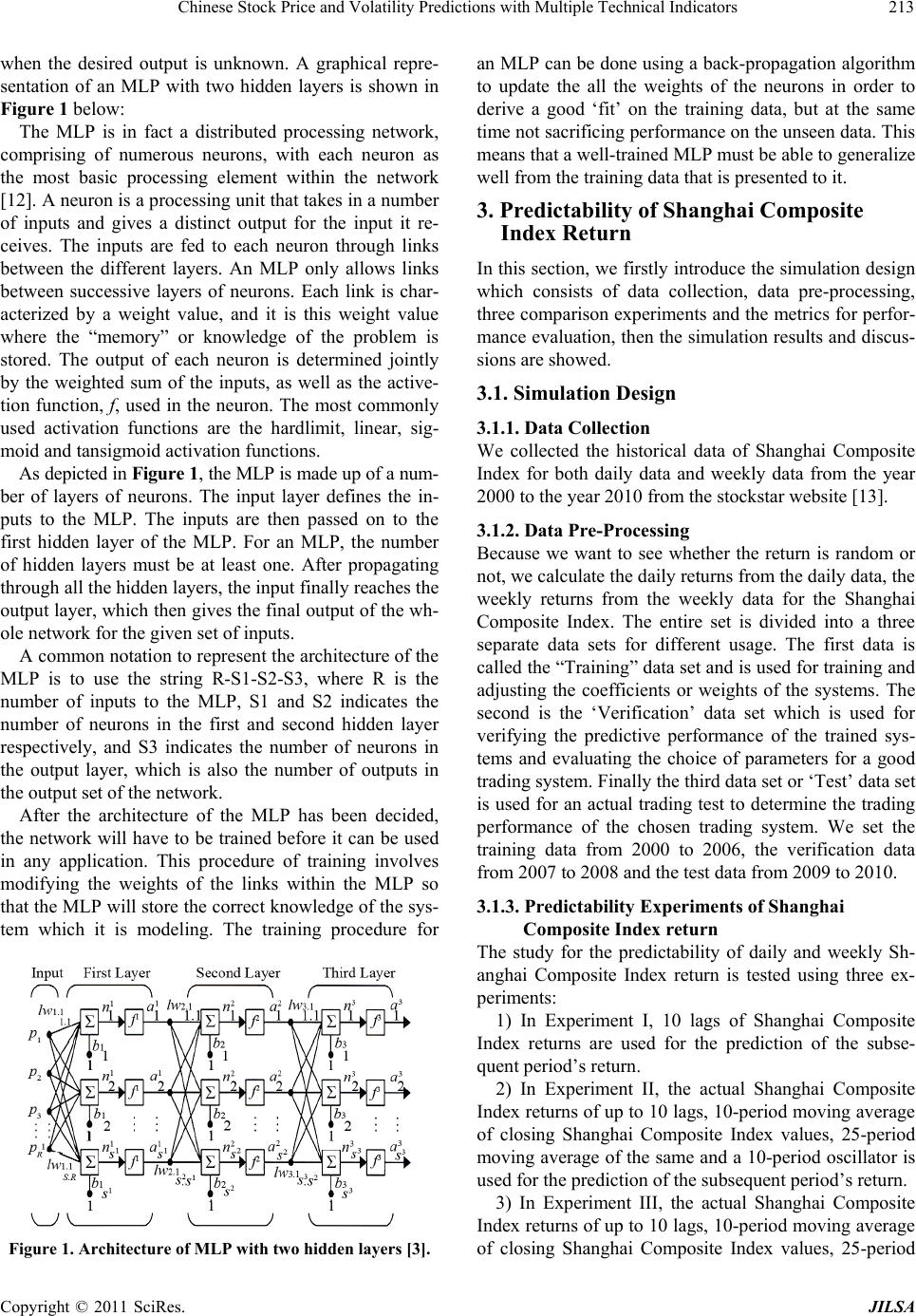hinese Stock Price and Volatility Predictions with Multiple Technical Indicators213
when the desired output is unknown. A graphical repre-
sentation of an MLP with two hidden layers is shown in
Figure 1 below:
The MLP is in fact a distributed processing network,
comprising of numerous neurons, with each neuron as
the most basic processing element within the network
[12]. A neuron is a processing unit that takes in a number
of inputs and gives a distinct output for the input it re-
ceives. The inputs are fed to each neuron through links
between the different layers. An MLP only allows links
between successive layers of neurons. Each link is char-
acterized by a weight value, and it is this weight value
where the “memory” or knowledge of the problem is
stored. The output of each neuron is determined jointly
by the weighted sum of the inputs, as well as the active-
tion function, f, used in the neuron. The most commonly
used activation functions are the hardlimit, linear, sig-
moid and tansigmoid activatio n functions.
As depicted in Figure 1, the MLP is made up of a num-
ber of layers of neurons. The input layer defines the in-
puts to the MLP. The inputs are then passed on to the
first hidden layer of the MLP. For an MLP, the number
of hidden layers must be at least one. After propagating
through all the hidden layers, the input finally reaches the
output layer, which then gives the final output of the wh-
ole network for the given set of inputs.
A common notation to represent the architecture of the
MLP is to use the string R-S1-S2-S3, where R is the
number of inputs to the MLP, S1 and S2 indicates the
number of neurons in the first and second hidden layer
respectively, and S3 indicates the number of neurons in
the output layer, which is also the number of outputs in
the output set of the network.
After the architecture of the MLP has been decided,
the network will have to be trained before it can be used
in any application. This procedure of training involves
modifying the weights of the links within the MLP so
that the MLP will store the correct kn owledge of the sys-
tem which it is modeling. The training procedure for
Figure 1. Architecture of MLP with two hidden layers [3].
an MLP can be done using a back -propagation algorithm
to update the all the weights of the neurons in order to
derive a good ‘fit’ on the training data, but at the same
time not sacrificing performance on the unseen data. This
means that a well-trained MLP must be able to g eneralize
well from the training data that is presented to it.
3. Predictability of Shanghai Composite
Index Return
In this section, we firstly introduce the simulation design
which consists of data collection, data pre-processing,
three comparison experiments and the metrics for perfor-
mance evaluation, then the simulation results and discus-
sions are showed.
3.1. Simulation Design
3.1.1. Dat a Collection
We collected the historical data of Shanghai Composite
Index for both daily data and weekly data from the year
2000 to the year 2010 from the stockstar website [13 ].
3.1.2. D ata Pre-Processing
Because we want to see whether the return is random or
not, we calculate the daily returns from the daily d ata, th e
weekly returns from the weekly data for the Shanghai
Composite Index. The entire set is divided into a three
separate data sets for different usage. The first data is
called the “Training ” data set and is used for training and
adjusting the coefficients or weights of the systems. The
second is the ‘Verification’ data set which is used for
verifying the predictive performance of the trained sys-
tems and evaluating the choice of parameters for a good
trading system. Finally the third data set or ‘Test’ data set
is used for an actual trading test to determine the trading
performance of the chosen trading system. We set the
training data from 2000 to 2006, the verification data
from 2007 to 2008 and the test data from 2009 to 2010.
3.1.3. Predictability Experiments of Shanghai
Composite Index return
The study for the predictability of daily and weekly Sh-
anghai Composite Index return is tested using three ex-
periments:
1) In Experiment I, 10 lags of Shanghai Composite
Index returns are used for the prediction of the subse-
quent peri od ’s ret ur n.
2) In Experiment II, the actual Shanghai Composite
Index return s of up to 10 lags, 10-period moving average
of closing Shanghai Composite Index values, 25-period
moving average of the same and a 10-period oscillato r is
used for the prediction of the subsequent period’s return.
3) In Experiment III, the actual Shanghai Composite
Index return s of up to 10 lags, 10-period moving average
of closing Shanghai Composite Index values, 25-period

Chinese Stock Price and Volatility Predictions with Multiple Technical Indicators
214
moving average of the same and a 10-period volatility
indicator is used for the prediction of the subsequent pe-
riod’s return.
In Experiments II and III, the term “period” refers to
daily or weekly based on the context of the experiment.
In each of the three experiments, the efficacy of the regr-
ession and neural network models in predicting the sub-
sequent period’s Shanghai Composite Index return is ev-
aluated.
3.1.4. Metrics Used for Performance E valuation
The performance of all the trading systems used in this
paper will be accessed using two metrics:
3.1.4.1. Di re ct ional Accura cy
The first metric is the percentage of correct signs of pre-
dicted returns as compared to the actual returns. This is
termed as directional accuracy in this paper. It has been
argued in literature that for prediction on the stock mar-
ket, the signs of returns are more important th an the actu-
al magnitude of returns. Also, it has been shown by Pesa-
ran and Timmermann [2] that directional accuracy meas-
ures has a higher correlation with returns compared to
using the mean square error.
3.1.4.2. Annual Return Rate
The second metric is the annual return rate (ARR) from
simulated trading. The ARR indicates the annual returns
from trading with an initial investment of 1 (ARR of 1.1
indicates a 10% profit). In this paper, both trading with
and without short selling has been considered. Also, both
the cases with and without commission costs are discu-
ssed to show the effects of commission costs when the
trading systems are in actual use. As mentioned earlier,
commission costs play a significant role when the num-
ber of transactions gets large.
In this paper, the commission cost is assumed to be
0.2% per trade (a single trade indicates either a buying or
selling decision), which is a rather conservative amount.
In computing the ARR for trading performance evalua-
tion, the cumulative return s for the who le period (training
or verification) is calculated first. After which, the ARR
is obtained by taking the nth root of the cumulative re-
turns, where n is the number of years in the period. In
calculating the cumulative returns, two possibilities exist
depending whether a lon g or short position is he ld. In the
case of a long position, the cumulative return after p eriod
t is calculated as:



Cumulative Returns
Cumulative Returns1Actual Returns
t
t
t
f


(9)
For a short position, the cumulative return in period t
is:


 
Cumu lative Returns
Cumu lative Re turns1Actual Returns
t
t
t

 (10)
For the tradin g decision made in this chapter, the thre-
shold-based trading rule is used. The threshold based tra-
ding rule is based on both the magnitude and signs of
predictions made by the systems. This decision-making
trading rule is used to make trading decisions via the fol-
lowing clauses:
1) If the predicted return rate is positive and its magni-
tude greater than the threshold value, then a long (buy)
position is recommended.
2) Alternatively, if the predicted return rate is negative
and its magnitude greater than the threshold, then a short
(sell) position is recommended.
3) If the above conditions fail, 3 scenarios are possible
whereby the recommendation is to stay away from the
market. If already in a long position, withdraw from mar-
ket if the predicted return rate is negative. On the other
hand, if already in a short position, withdraw from mar-
ket if the return rate is positive. Else, the current position
is maintained.
The use of this threshold-based trading rule leads to
the need to vary the threshold value used in order to find
an appropriate value for the trading system which leads
to good trading p erformances.
3.2. Simulation Results
3.2.1. Predictability Experiments of Shanghai
Composite Index Return
For convenience, in the presentation of tables, we denote
directional accuracy as DA, annual return rate as ARR
and commission fee as CF.
For daily data, we firstly use the regression model to
do the prediction. We show the experiment results in Ta-
bles 1-3:
Table 1. Performance of regression model in experiment I
(daily).
ARR (No short sell)ARR (Short sell)
Period DA No CF 0.2% CFNo CF0.2% CF
Training 54.21%1.2879 1.2760 1.25791.2330
Verification 54.81%1.0698 1.0511 1.71731.6586
Table 2. Performance of regression model in experiment II
(daily).
ARR (No short sell)ARR (Short sell)
Period DA No CF 0.2% CFNo CF0.2% CF
Training 52.90%1.2154 1.1960 1.28551.2462
Verification55.65%0.9676 0.9620 1.45071.4336

Chinese Stock Price and Volatility Predictions with Multiple Technical Indicators215
In experiment I, the threshold for trading is 0.0008. In
experiment II, the threshold for trading is 0.0002. In ex-
periment III, the threshold for trading is 0.0006. From the
Tables 1-3, we can see that the experiment I showed the
best performance of regression model. So we choose the
method in experiment I for test period. We show the re-
sult in Table 4.
In experiment I, the threshold for trading is 0.0018 and
the number of nodes is 18. In experiment II, the threshold
for trading is 0.0016 and the number of nodes is 18. In
experiment III, the threshold for trading is 0.0014 and the
number of nodes is 12. From the Tab les 5-7, we can see
that the experiment II showed the best performance of
NN model. So we choose the method and parameters in
experiment II for test period. We show the result in Ta-
ble 8.
Table 3. Performanc e of regression model in experime nt III
(daily).
ARR (No short sell)ARR (Short sell)
Period DA No CF 0.2% CFNo CF0.2% CF
Training 53.68%1.2690 1.2581 1.39551.3714
Verification 57.11%0.9434 0.9380 1.12351.1116
Table 4. Performance of regression model in experiment I
(daily).
ARR (No short sell)ARR (Short sell)
Period DA No CF 0.2% CFNo CF0.2% CF
Testing 56.63%1.2638 1.2572 1.33511.3299
Table 5. Performance of NN model in experiment I (daily).
ARR (No short sell)ARR (Short sell)
Period DA No CF 0.2% CFNo CF0.2% CF
Training 55.89%1.4654 1.4458 1.83841.7981
Verification 55.86%1.1324 1.1118 1.71821.6624
Table 6. Performance of NN model in experiment II (daily).
ARR (No short sell)ARR (Short sell)
Period DA No CF 0.2% CFNo CF0.2% CF
Training 58.88%1.7051 1.6812 2.15712.1003
Verification 55.60%1.0135 1.0032 1.22611.2026
Table 7. Performance of NN model in exp eriment III (d aily).
ARR (No short sell)ARR (Short sell)
Period DA No CF 0.2% CFNo CF0.2% CF
Training 55.37%1.3453 1.3325 1.47821.4493
Verification 55.81%0.9581 0.9527 1.25541.2419
For the weekly data, we firstly use the regression mo-
del to do the prediction. We show the experiment results
in Tables 9-11.
In experiment I, the threshold for trading is 0.0014. In
experiment II, the threshold for trading is 0.0008. In ex-
periment III, the threshold for trading is 0.0002. From the
Tables 9-11 above, we can see that the experiment II
showed the best performance of regression model. So we
choose the method in experiment III for test period. We
show the result in Table 12 below.
Table 8. Performance of NN model in experiment II (daily).
ARR (No short sell)ARR (Short sell)
Period DA No CF 0.2% CFNo CF0.2% CF
Testing 56.02%1.2984 1.2569 1.39661.3517
Table 9. Performance of regression model in experiment I.
(weekl y)
ARR (No short sell)ARR (Short sell)
Period DA No CF 0.2% CFNo CF0.2% CF
Training 62.86%1.2441 1.2416 1.36131.3563
Verification 56.67%1.0308 1.0287 1.47731.4711
Table 10. Performance of regression model in experiment II
(weekly).
ARR (No short sell)ARR (Short sell)
Period DA No CF 0.2% CFNo CF0.2% CF
Training 59.40%1.2398 1.2356 1.37351.3646
Verification 66.67%1.1800 1.1781 1.70991.7048
Table 11. Performance of regression model in experiment
III (weekly).
ARR (No short sell)ARR (Short sell)
Period DA
No CF 0.2% CFNo CF0.2% CF
Training 59.06%1.1035 1.0980 1.10131.0902
Verification 44.57%0.8628 0.8590 0.93030.9221
Table 12. Performance of regression model in experiment II
(weekly).
ARR (No short sell)ARR (Short sell)
Period DA No CF 0.2% CFNo CF0.2% CF
Testing 55.25%0.9054 0.9039 0.90200.8988

Chinese Stock Price and Volatility Predictions with Multiple Technical Indicators
216
For the weekly data, we then use the NN model to do
the prediction. We show the experiment results in Tables
13-15.
In experiment I, the threshold for trading is 0.0010 and
the number of nodes is 14. In experiment II, the threshold
for trading is 0.0020 and the number of nodes is 12. In
experiment III, the threshold for trading is 0.0014 and the
number of nodes is 20. From the Table 13 ~ 15, we can
see that the experiment II showed the best performance
of NN model. So we choose the method and parameters
in experiment II for test period. We show the result in
Table 16.
From the results showed above, we can see that the
performance of NN model is better than the performance
of regression model. We also can find that for the daily
data, the ARRs of both regression model and NN model
are better than the ARRs of buy-and-hold strategy in
testing period (testing period ARR is 1.2419). Unfortu-
nately, for the weekly data, the ARRs of both regression
model and NN model are worse than the ARRs of buy-
and-hold strategy.
Table 13. Performance of NN model in experiment I (weekly).
ARR (No short sell)ARR (Short sell)
Period DA No CF 0.2% CFNo CF0.2% CF
Training 66.29%1.4186 1.4122 1.68721.6728
Verification 53.33%1.0847 1.0795 1.52571.5108
Table 14. Performance of NN model in experiment II (week-
ly).
ARR (No short sell)ARR (Short sell)
Period DA No CF 0.2% CFNo CF0.2% CF
Training 62.39%1.3135 1.3081 1.43471.4242
Verification 56.67%1.0496 1.0480 1.33801.3337
Table 15. Performance of NN model in experiment III (week-
ly).
ARR (No short sell)ARR (Short sell)
Period DA No CF 0.2% CFNo CF0.2% CF
Training 65.63%1.1271 1.1237 1.17441.1673
Verification 52.17%1.0074 1.0039 1.13901.1313
Table 16. Performance of NN model in experiment II (week-
ly).
ARR (No short sell)ARR (Short sell)
Period DA No CF 0.2% CFNo CF0.2% CF
Testing 62.77%1.0613 1.0598 1.22871.2258
4. Predictability of Shanghai Composite
Index Price Volatility
In this section, we firstly introduce the simulation design
which consists of data collection, data pre-processing,
three comparison experiments and the metrics for perfor-
mance evaluation, then the simulation results and discus-
sions are showed.
4.1. Simulation Design
4.1.1. Dat a Collection
We collected the historical data of Shanghai Composite
Index for both daily data and weekly data from the year
2000 to the year 2010 from the stockstar website [13].
4.1.2. D ata Pre-Processing
Because we want to see whether the return is random or
not, we calculate the daily returns from the daily data, the
weekly returns from the weekly data for the Shanghai
Composite Index. The entire set is divided into a three
separate data sets for different usage. The first data is
called the “Training ” data set and is used for training and
adjusting the coefficients or weights of the systems. The
second is the “Verification” data set which is used for ve-
rifying the predictive performance of the trained systems
and evaluating the choice of parameters for a good trad-
ing system. Finally the third data set or “Test” da ta set is
used for an actual trading test to determine the trading
performance of the chosen trading system. We set the
training data from 2000 to 2006, the verification data
from 2007 to 2008 and the test data from 2009 to 2010.
4.1.3. Predictability Experiments of Shanghai
Composite Index Price Volatility
The study for the predictability of daily and weekly
Shanghai Composite Index price-changes is tested using
three experiments:
1) In Experiment IV, 10 lags of actual Shanghai Com-
posite Index closing price values and 10 lags of periodic
price-changes are used for the prediction of the subse-
quent period’s price-c hange.
2) In Experiment V, 10 lags of actual Shanghai Com-
posite Index trading volume values AND 10 lags of pe-
riodic trading volume differences are used for the predic-
tion of the subsequent period’s price-change.
3) In Experiment VI, 10 lags of actual Shanghai Com-
posite Index closing price values, 10 lags of periodic
price-changes, 10 lags of trading volume values and 10
lags of periodic trading volume differences are used for
the prediction of the subsequent period’s price change.
4.1.4. Metrics Used for Performance E valuation
The performance of all the trading systems used in this
paper will be accessed only using one metric:

C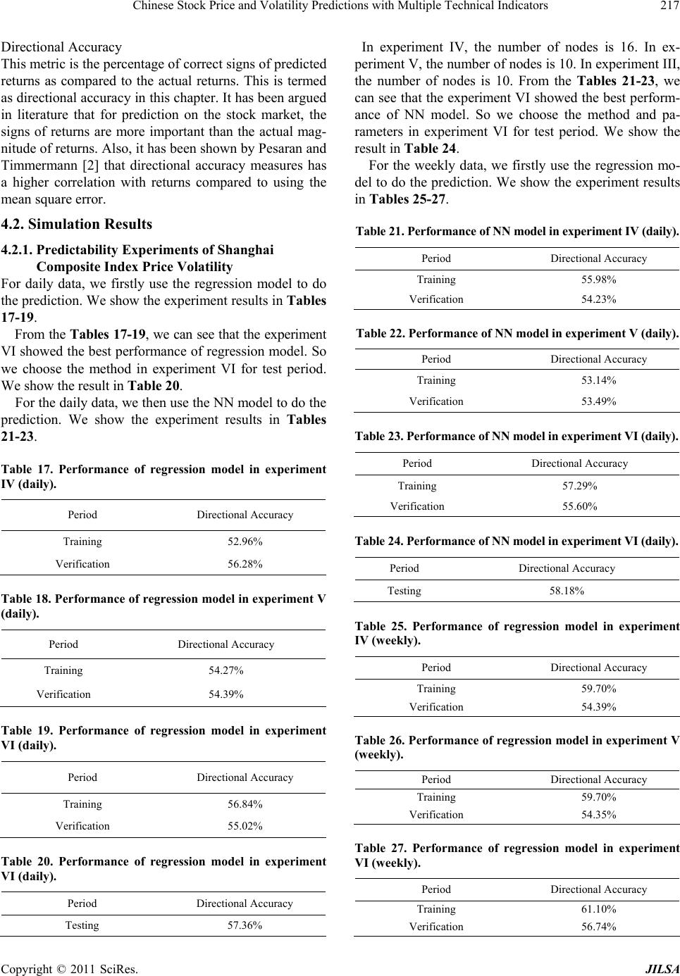hinese Stock Price and Volatility Predictions with Multiple Technical Indicators217
Directional Accuracy
This metric is the percentage of correct signs of predicted
returns as compared to the actual returns. This is termed
as directional accuracy in this chapter. It has been argued
in literature that for prediction on the stock market, the
signs of returns are more important than the actual mag-
nitude of returns. Also, it has been shown by Pesaran and
Timmermann [2] that directional accuracy measures has
a higher correlation with returns compared to using the
mean square error.
4.2. Simulation Results
4.2.1. Predictability Experiments of Shanghai
Composite Index Price Volatility
For daily data, we firstly use the regression model to do
the prediction. We show the experiment results in Tables
17-19.
From the Tables 17-19, we can see that the experiment
VI showed the best performance of regression model. So
we choose the method in experiment VI for test period.
We show the result in Table 20.
For the daily data, we then use the NN model to do the
prediction. We show the experiment results in Tables
21-23.
Table 17. Performance of regression model in experiment
IV (daily).
Period Directional Accuracy
Training 52.96%
Verification 56.28%
Table 18. Performance of re gression model in experiment V
(daily).
Period Directional Accuracy
Training 54.27%
Verification 54.39%
Table 19. Performance of regression model in experiment
VI (daily).
Period Directional Accuracy
Training 56.84%
Verification 55.02%
Table 20. Performance of regression model in experiment
VI (daily).
Period Directional Accuracy
Testing 57.36%
In experiment IV, the number of nodes is 16. In ex-
periment V, the number of nodes is 10. In experiment III,
the number of nodes is 10. From the Tables 21-23, we
can see that the experiment VI showed the best perform-
ance of NN model. So we choose the method and pa-
rameters in experiment VI for test period. We show the
result in Table 24.
For the weekly data, we firstly use the regression mo-
del to do the prediction. We show the experiment results
in Tables 25-27.
Table 21. Performance of NN model in experiment IV (daily).
Period Directional Accuracy
Training 55.98%
Verification 54.23%
Table 22. Performance of NN mod el in exp eriment V (daily).
Period Directional Accuracy
Training 53.14%
Verification 53.49%
Table 23. Performance of NN model in experiment VI (d aily).
Period Directional Accuracy
Training 57.29%
Verification 55.60%
Table 24. Performance of NN model in experiment VI (d aily).
Period Directional Accuracy
Testing 58.18%
Table 25. Performance of regression model in experiment
IV (weekly).
Period Directional Accuracy
Training 59.70%
Verification 54.39%
Table 26. Performance of re gression model in experiment V
(weekly).
Period Directional Accuracy
Training 59.70%
Verification 54.35%
Table 27. Performance of regression model in experiment
VI (weekly).
Period Directional Accuracy
Training 61.10%
Verification 56.74%

C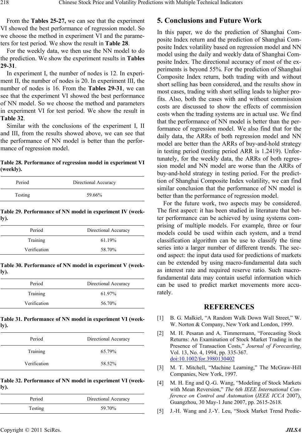hinese Stock Price and Volatility Predictions with Multiple Technical Indicators
218
From the Tables 25-27, we can see that the experiment
VI showed the best performance of regression model. So
we choose the method in experiment VI and the parame-
ters for test period. We show the result in Table 28.
For the weekly data, we then use the NN model to do
the prediction. We show the experiment results in Tables
29-31.
In experiment I, the number of nodes is 12. In experi-
ment II, the number of nodes is 20. In experiment III, the
number of nodes is 16. From the Tables 29-31, we can
see that the experiment VI showed the best performance
of NN model. So we choose the method and parameters
in experiment VI for test period. We show the result in
Table 32.
Similar with the conclusions of the experiment I, II
and III, from the results showed above, we can see that
the performance of NN model is better than the perfor-
mance of regression model.
Table 28. Performance of regression model in experiment VI
(weekly).
Period Directional Accuracy
Testing 59.66%
Table 29. Performance of NN model in experiment IV (week-
ly).
Period Directional Accuracy
Training 61.19%
Verification 58.70%
Table 30. Performance of NN model in experime nt V (wee k-
ly).
Period Directional Accuracy
Training 61.97%
Verification 56.70%
Table 31. Performance of NN model in experiment VI (week-
ly).
Period Directional Accuracy
Training 65.79%
Verification 58.52%
Table 32. Performance of NN model in experiment VI (week-
ly).
Period Directional Accuracy
Testing 59.70%
5. Conclusions and Future Work
In this paper, we do the prediction of Shanghai Com-
posite Index return and the prediction of Shanghai Com-
posite Index volatility based on regression model and NN
model using the daily and weekly data of Shanghai Com-
posite Index. The directional accuracy of most of the ex-
periments is beyond 55%. For the prediction of Shanghai
Composite Index return, both trading with and without
short selling has been considered, and the results show in
most cases, trading with short selling leads to high er pro-
fits. Also, both the cases with and without commission
costs are discussed to show the effects of commission
costs when the trading systems are in actual use. We find
that the performance of NN model is better than the per-
formance of regression model. We also find that for the
daily data, the ARRs of both regression model and NN
model are better than the ARRs of buy-and-hold strategy
in testing period (testing period ARR is 1.2419). Unfor-
tunately, for the weekly data, the ARRs of both regres-
sion model and NN model are worse than the ARRs of
buy-and-hold strategy in testing period. For the predict-
tion of Shanghai Composite Index volatility, we can find
similar conclusion that the performance of NN model is
better than the performance of regression model.
For the future work, two aspects may be considered.
The first aspect: it has been studied in literature that bet-
ter performance can be achieved by using systems com-
prising of multiple models. For example, three or four
models could be used within each system, and a trend
classification algorithm can be use to classify the time
series into a larger number of different trends. The sec-
ond aspect: the input data used for predictions of markets
can be extended by using macro-fundamental data such
as interest rate and required reserve ratio. Such macro-
fundamental data may contain useful information which
can be used to predict market movements more accu-
rately.
REFERENCES
[1] B. G. Malkiel, “A Random Walk Down Wall Street,” W.
W. Norton & Company, New York and London, 1999.
[2] M. H. Pesaran and A. Timmermann, “Forecasting Stock
Returns: An Examination of Stock Market Trading in the
Presence of Transaction Costs,” Journal of Forecasting,
Vol. 13, No. 4, 1994, pp. 335-367.
doi:10.1002/for.3980130402
[3] M. T. Mitchell, “Machine Learning,” The McGraw-Hill
Companies, New York, 1997.
[4] M. H. Eng and Q.-G. Wang, “Modeling of Stock Markets
with Mean Reversion,” The 6th IEEE International Con-
ference on Control and Automation (IEEE ICCA 2007),
Guangzhou, 30 May-1 June 2007, pp. 2615-2618.
[5] J.-H. Wang and J.-Y. Leu, “Stock Market Trend Predic-

Chinese Stock Price and Volatility Predictions with Multiple Technical Indicators
219
tion Using ARIMA-Based Neural Networks,” The 1996
IEEE International Conference on Neural Networks, Wa-
shington DC, 3-6 June 1996, pp. 2160-2165.
[6] W. Wang, D. Okunbor and F. C. Lin, “Future Trend of
the Shanghai Stock Market,” ICONIP '02: Proceedings of
the 9th International Conference on Neural Information
Processing, Singapore, 18-22 November, pp. 2320-2324.
[7] L.-X. Liu and J.-H Ma, “Multivariate Nonlinear Predic-
tion of Shenzhen Stock Price,” The 3rd International
Conference on Wireless Communications, Networking and
Mobile Computing (WiCOM 2007), Shanghai, 21-23 Sep-
tember 2007, pp. 4120-4123.
[8] S.-H. Chen, C.-Q Tao and W. He, “A New Algorithm of
Neural Network and Prediction in China Stock Market,”
Pacific-Asia Conference on Circuits, Communications
and Systems, PACCS 2009, Chengdu, 16-17 May 2009,
pp. 686-689.
[9] X. Xiong, X,-T, Zhang, W, Zhang and C,-Y, Li, “Wave-
let-Based Beta Estimation of China Stock Market,” Pro-
ceedings of 2005 International Conference on Machine
Learning and Cybernetics, Guan gzhou, 18-21 Aug ust 2005,
pp. 3501-3505.
[10] W.-R. Pan, “Empirical Analysis of Stock Returns Vola-
tility in China Market Based on Shanghai and Shenzhen
300 Index,” 2010 International Conference on Financial
Theory and Engi neering (ICFTE), Dubai, 18-20 June 2010,
pp. 17-21.
[11] X.-M. Song and H.-X. Pan, “Analysis of China Stock
Market: Volatility and Influencing Factors,” 2010 Inter-
national Conference on Management and Service Science
(MASS), Wuhan, 24-26 August 2010, pp. 1-5.
doi:10.1109/ICMSS.2010.5578224
[12] S. Haykin, “Neural Networks: A Comprehensive Founda-
tion”, Prentice-Hall, Saddle River, 1999.
[13] Http://www.stockstar.com/