Journal of Mathematical Finance, 2011, 1, 109-119
doi:10.4236/jmf.2011.13014 Published Online November 2011 (http://www.SciRP.org/journal/jmf)
On Value Premium, Part I: The Existence
Chi Fung Ling1, Simon Gar Man Koo2
1Department of Industrial Engineering and Operations Research, Columbia University, New York, USA
2Department of Mathematics and Computer Science, University of San Diego, San Diego, USA
Received August 28, 2011; revised September 14, 2011; accepted September 22, 2011
Abstract
A great deal of academic research provides solid evidence that value investing generated better returns than
growth investing from the early 1970s to the mid-1990s. However, the relatively poor performance of value
stocks in the late 1990s generated suspicion that value investing was failing. Such claims were invalidated by
empirical research showing that value stocks’ slump in this period was not caused by a change in fundamen-
tal patterns, but rather by investors’ overly-rosy expectations for new technology companies.
Keywords: Value Investing, Value Premium, Growth Stocks, Value Stocks, Beta, Downside Risk,
Systematic Risk
1. Introduction
The foundation of value investing dates back to [1] in
which Graham and Dodd argued that securities should be
purchased if their market price is less than their intrinsic
value. Since then, this trading strategy has received much
attention from investors and academics alike. Basu [2]
showed that stocks with low p rice-to-earnings ratio s (P/E)
tend to have higher subsequent average returns than
stocks with high P/E. They called this return “the value
premium”. Echoing the result of [2], Fama and French [3 ]
and Lakonishok, Shleifer, and Vishny [4] provided em-
pirical evidence that the returns of value investing don’t
follow the beta rule in the Capital Asset Pricing Model,
sparking debate about the death of beta.
On the other hand, Chan, Hamao, and Lakonishok [5]
showed that the value premium also existed in Japan’s
stock market. Fama and French [6] further confirmed that
value stocks outperformed growth stocks in all major
financial markets.
This academic work has had a tremendous impact on
the investment industry. Not only has value investing been
widely adopted by portfolio managers, b ut ratios like the
book value to market value of equity (BV/MV) has also
become an important indicator of managers’ investment
strategy orientation.
Given the significance of value investing, this paper
will be surveying empirical academic evidence for value
premium. Note that the late-1990s equity market perfor-
ma nce has always b een used as a forcefu l counterargument
to the existenc e of value pr emium. We will, however , show
that even if we include the late-1990s stocks’ perform-
ance, value investing had still generated superior returns.
2. Proof of the Existence of Value Premium
2.1. Evidence
Us ing stocks’ data from 1963 to 1990 f rom CRSP-COMU-
STAT Fama and French [3] sorted stocks into 10 portfo-
lios according t o their B ook Value/ Market Value (B V/MV).
They further split the top and bottom decile portfolios
into equal halves. In Table 1, one can see that the top de-
cile portfolios (10A and 10B) have the highest BV/MV
and are termed the “value portfolios.” Market generally
deems that value portfolios are stocks with little (earn-
ings) growth in the past and will continue such trend in
the future. The bottom decile portfolios (1A and 1B)
have the lowest BV/MV and are termed “glamour/growth
portfolios.” They have opposite properties to that of value
portfoli os. T he st ocks in ea ch port foli o ar e equ ally wei ghted
and the portfolio is reconstructed each year according to
the stocks’ BV/MV. The result is shown in Table 1, Panel
A. One can see that the value portfolio (10B) generated
an average monthly return of 1.83%, compared to 0.3%,
fo r the glamour portfolio (1A), making for a 1.53% sp read.
One can also notice that their betas are very close to each
other (1.35 vs. 1.36), supporting the idea that systematic
risk cannot be attributed to this spread. However, some
other measures of risk have to be taken into account before

C. F. LING ET AL.
110
Table 1. Excerpt from Fama and French (1992)—Properties of portfolios formed on Book-to-Market Equity (BE/ME) and
Earnings-Price Ratio (E/P), 1963-1990.
Portfolio 0 1A 1B 2 3 4 5 6 7 8 9 10A 10B
Panel A: Stocks Sorted on Book-to-Market E quity (BE/ME)
Return 0.30 0.67 0.87 0.97 1.04 1.17 1.30 1.44 1.50 1.59 1.92 1.83
β 1.36 1.34 1.32 1.30 1.28 1.27 1.27 1.27 1.27 1.29 1.33 1.35
ln(ME) 4.53 4.67 4.69 4.56 4.47 4.38 4.23 4.06 3.85 3.51 3.06 2.65
ln(BE/ME) –2.22 –1.51 –1.09 –0.75–0.51–0.32–0.14 0.03 0.21 0.42 0.66 1.02
ln(A/ME) –1.24 –0.79 –0.40 –0.050.20 0.40 0.56 0.71 0.91 1.12 1.35 1.75
ln(A/BE) 0.94 0.71 0.68 0.70 0.71 0.71 0.70 0.68 0.70 0.70 0.70 0.73
E/P dummy 0.29 0.15 0.10 0.08 0.08 0.08 0.09 0.09 0.11 0.15 0.22 0.36
E(+)/P 0.03 0.04 0.06 0.08 0.09 0.10 0.11 0.11 0.12 0.12 0.11 0.10
Firms 89 98 209 222 226 230 235 237 239 239 120 117
Portfolio 0 1A 1B 2 3 4 5 6 7 8 9 10A 10B
Panel B: Stocks Sorted on Earnings-Price Ratio (E/P)
Return 1.46 1.04 0.93 0.94 1.03 1.18 1.22 1.33 1.42 1.46 1.57 1.74 1.72
β 1.47 1.40 1.35 1.31 1.28 1.26 1.25 1.26 1.24 1.23 1.24 1.28 1.31
ln(ME) 2.48 3.64 4.33 4.61 4.64 4.63 4.58 4.49 4.37 4.28 4.07 3.82 3.52
ln(BE/ME) –0.10 –0.76 –0.91 –0.79 –0.61–0.47–0.33–0.21–0.08 0.02 0.15 0.26 0.40
ln(A/ME) 0.90 –0.05 –0.27 –0.16 0.03 0.18 0.31 0.44 0.58 0.70 0.85 1.01 1.25
ln(A/BE) 0.99 0.70 0.63 0.63 0.64 0.65 0.64 0.65 0.66 0.68 0.71 0.75 0.86
E/P dummy 1.00 0.00 0.00 0.00 0.00 0.00 0.00 0.00 0.00 0.00 0.00 0.00 0.00
E(+)/P 0.00 0.01 0.03 0.05 0.06 0.08 0.09 0.11 0.12 0.14 0.16 0.20 0.28
Firms 355 88 90 182 190 193 196 194 197 195 195 95 91
At the end of each year t – 1, 12 portfolios are formed on the basis of ranked values of BE/ME or E/P. Portfolios 2 - 9 cover deciles of the ranking variables.
The bottom and top 2 portfolios (1A, 1B, 10A, and 10B) split the bottom and top deciles in half. For E/P, there are 13 portfolios; portfolio 0 is stocks with
negative E/P. Since BE/ME and E/P are not strongly related to the exchange listing, their portfolio breakpoints are determined on the basis of the ranked values
of the variables for all stocks that satisfy the CRSP-COMPUSTAT data requirements. BE is the book value of common equity plus balance-sheet deferred taxes,
A is total book assets, and E is ear ni n gs (income before ext raordinary i t ems, plus income-statement deferred taxes, minus preferred dividends). BE, A, and E are
for each f ir m’s l ates t fi scal y ear en di ng i n cal end ar y ear t – 1. The accounting ratios are measured using market equity ME in December of year t – 1. Firm size
ln(ME) is measured in June of year t + 1, and then reform the portfolios at the end of year t. Return is the t ime-series aver age of the mon thly equal- weighted
portfolio returns (in percent). ln(ME), ln(BE/ME), ln(A/ME), ln(A/BE), E(+)/P, and E/P dummy are t he time-s eries averag es of th e monthly av erage v alues of
these var i ab l es in each portfo l io . S in ce t he E/P dummy is 0 when earn i ngs are posi ti ve, and 1 when earnings are negative, E/P dummy gives th e av er age propor -
tion of stocks with negative earnings in each portfolio. β is the time-series average of the monthly portfolio β s. Stocks ar e assigned t he post-ra nking β of the size-
β portfolio they are in at the end of June of year t (Table É). These individual-firm β s are averages to compute the monthly β s for each portfolio for July of year
t to June of year t + 1. Firms is the average number of stocks in the portfolio each month.
we can determine conclusively that value stocks are not
fundamentally riskier. Notice that the logarithm of MV for
the value portfolio is 2.65, compared to 4.53 for the gla-
mour portfolio. This indicates the differences in sizes of
the portfol ios’ mar ket equity. A ccording to [7], the stock o f
a small fir m wi ll always h ave a pre mium co mpared to that
of a big firm, and this may contribute to spread.
Echoing the results of [3], Lakonishok, Shleifer, and
Vishny [4] conducted similar empirical research using
data from 1968 to 1989, and the results are shown in Ta-
ble 2, Panel A. Instead of re-forming the portfolios each
year, they used a buy-and-hold strategy: after construct-
ing a portfolio, it is held for five years, and the average
return is calculated annu ally. The goal of doing that is to
evaluate the return of value investment in long term. One
can see that the average annual return (“AR” in the table)
of the value portfolio is 19.8% compared to 9.3% of the
glamour portfolio, a 10.5% spread. To take the factor of
size into account, the average annual sized-adjusted re-
turn (“SAAR”) is also included in this table. After ad-
justing for size, the superiority of the value portfolio’s
returns persists even though the gap is now smaller: its
SAAR is 3.5%, compared to –4.3% for the glamour port-
folio, a 7.8% spread. This shows that part of the spread
may be attributed to the size of equity.
Another proof came from [3] in which they compared
the average monthly return of only large cap stocks. Again,
they ranked stocks according to their BV/MV within this
large-cap criterion and created 10 portfolios. The return
of each portfolio is shown in Table 3 under the row

111 C. F. LING ET AL.
Table 2. Excerpt from Lakonishok, Shleifer, and Vish ny (1994)—Re turns for de cile portfolios based on one- dimensional clas-
sificiations by various measures of value, 1968-1989.
Glamour Value
1 2 3 4 5 6 7 8 9 10
Panel A: B/M
R1 0.0110 0.117 0.135 0.123 0.131 0.154 0.154 0.170 0.183 0.173
R2 0.079 0.107 0.140 0.145 0.153 0.156 0.169 0.164 0.182 0.188
R3 0.107 0.132 0.155 0.167 0.165 0.172 0.191 0.207 0.196 0.204
R4 0.081 0.133 0.136 0.160 0.170 0.169 0.188 0.204 0.213 0.207
R5 0.088 0.137 0.163 0.175 0.171 0.176 0.216 0.201 0.206 0.215
AR 0.093 0.125 0.146 0.154 0.158 0.166 0.184 0.189 0.196 0.198
CR5 0.560 0.802 0.973 1.045 1.082 1.152 1.320 1.375 1.449 1.462
SAAR –0.043 –0.020 –0.003 0.004 0.006 0.012 0.024 0.028 0.033 0.035
Panel B: C/P
R1 0.084 0.124 0.140 0.140 0.153 0.148 0.157 0.178 0.183 0.183
R2 0.067 0.108 0.126 0.153 0.156 0.170 0.177 0.180 0.183 0.190
R3 0.096 0.133 0.153 0.172 0.170 0.191 0.191 0.202 0.193 0.204
R4 0.098 0.111 0.146 0.159 0.166 0.172 0.182 0.192 0.223 0.218
R5 0.108 0.134 0.161 0.162 0.187 0.177 0.191 0.209 0.212 0.208
AR 0.091 0.122 0.145 0.157 0.166 0.171 0.180 0.192 0.199 0.201
CR5 0.543 0.779 0.969 1.074 1.158 1.206 1.283 1.406 1.476 1.494
SAAR –0.049 –0.025 –0.006 0.005 0.013 0.019 0.025 0.034 0.037 0.039
Panel C: E/P
R1 0.123 0.125 0.140 0.130 0.135 0.156 0.170 0.180 0.193 0.162
R2 0.101 0.113 0.124 0.143 0.167 0.164 0.180 0.185 0.183 0.174
R3 0.118 0.138 0.157 0.171 0.171 0.191 0.198 0.188 0.188 0.195
R4 0.111 0.124 0.145 0.151 0.157 0.159 0.198 0.199 0.205 0.214
R5 0.119 0.129 0.151 0.167 0.171 0.168 0.196 0.201 0.211 0.207
AR 0.114 0.126 0.143 0.152 0.160 0.167 0.188 0.191 0.196 0.190
CR5 0.717 0.808 0.953 1.031 1.102 1.168 1.370 1.393 1.446 1.388
SAAR –0.035 –0.024 –0.009 –0.001 0.005 0.013 0.026 0.026 0.029 0.019
Panel D: GS
Value Glamour
1 2 3 4 5 6 7 8 9 10
R1 0.187 0.183 0.164 0.169 0.162 0.157 0.159 0.164 0.142 0.114
R2 0.181 0.180 0.186 0.169 0.166 0.162 0.152 0.157 0.147 0.131
R3 0.204 0.206 0.194 0.186 0.181 0.180 0.168 0.178 0.157 0.138
R4 0.205 0.193 0.201 0.190 0.181 0.174 0.160 0.153 0.167 0.126
R5 0.197 0.213 0.194 0.199 0.168 0.184 0.185 0.168 0.163 0.125
AR 0.195 0.195 0.188 0.183 0.171 0.171 0.165 0.164 0.155 0.127
CR5 1.434 1.435 1.364 1.314 1.205 1.206 1.144 1.136 1.057 0.818
SAAR 0.022 0.027 0.025 0.024 0.015 0.015 0.008 0.008 0.000 –0.024
At the end of each April between 1968 and 1989, 10-decile portfolios are formed in ascending order based on B/M, C/P, E/P, and GS. B/M is the ratio of book
value of equity to market value of equity; C/P is the ratio of cash flow to market value of equity; E/P is the ratio of earnings to market value of equity, and GS
refers t o prefor mation 5-year average g rowt h rate of s ales. The ret urns pr esented i n the tab le are av erages o ver all format ion periods. Rt is the av erage ret urn in
year t after formation, t = 1, ···, 5. AR is the average annual return over 5 postformation years. CR5 is the compounded 5-year return assuming annual rebalanc-
ing. SAAR is the average annual size-adjusted return computed over 5 postformation years. The glamour portfolio refers to the decile portfolio containing
stocks ranking lowest on B/M, C/P, or E/P, or highest on GS. The value portfolio refers to the decile portfolio contai ni ng stocks ranking highest on B/M, C/P, or
E/P, or lowest on GS.

C. F. LING ET AL.
112
Table 3. Excerpt from Fama and French (1992)—Average monthly returns on portfolios formed on size and Book-to-Market;
Stocks Sorted by ME (Down) and then BE/ME (Across), 1963-1990.
Book-to-Market Portfolios
All Low 2 3 4 5 6 7 8 9 High
All 1.23 0.64 0.98 1.06 1.17 1.24 1.26 1.39 1.40 1.50 1.63
Small-ME 1.47 0.7 1.14 1.20 1.43 1.56 1.51 1.70 1.71 1.82 1.92
ME-2 1.22 0.43 1.05 0.96 1.19 1.33 1.19 1.58 1.28 1.43 1.79
ME-3 1.22 0.56 0.88 1.23 0.95 1.36 1.30 1.30 1.40 1.54 1.60
ME-4 1.19 0.39 0.72 1.06 1.36 1.13 1.21 1.34 1.59 1.51 1.47
ME-5 1.24 0.88 0.65 1.08 1.47 1.13 1.43 1.44 1.26 1.52 1.49
ME-6 1.15 0.7 0.98 1.14 1.23 0.94 1.27 1.19 1.19 1.24 1.50
ME-7 1.07 0.95 1.00 0.99 0.83 0.99 1.13 0.99 1.16 1.10 1.47
ME-8 1.08 0.66 1.13 0.91 0.95 0.99 1.01 1.15 1.05 1.29 1.55
ME-9 0.95 0.44 0.89 0.92 1.00 1.05 0.93 0.82 1.11 1.04 1.22
Large-ME 0.89 0.93 0.88 0.84 0.71 0.79 0.83 0.81 0.96 0.97 1.18
In June of each year t, the NYS E, AMEX, and NASDAQ stock s that meet the CRSP -COMPUSTAT data requ irements are allo cated to 10 size portfolio s using
the NYSE size (ME) br eakpoints. Th e NYSE, AMEX, and NAS DAQ stocks in each size d ecile then sorted into 10 BE/ME portfolios usin g the book-to-market
ratios for year t – 1, over t he market equ ity for December of year t – 1. The equal-weighted monthly portfolio returns are then calculated for July of year t to
June of year t + 1. Average monthly return is the time-series average of the monthly equal-weighted portfolio returns (in percent). The All column shows aver-
age returns for equal-weighted size decile portfolios. The All row shows average returns for equal-weighted portfolios of the stocks in each BE/ME group.
LARGE-ME. Notice that the average monthly return for
the value stocks is 1.18% compared to 0.89% for the
glamour stocks, a 0.29% spread. The spread still exists
but it is less substantial. Combining the studies above
lead us to conclude that part of the spread may be attrib-
ute to the size of equity. But the spread still exists even if
we take the size factor into account and this could be due
to the value premium.
Research was also conducted to see if ano ther measure
could be used to create a similar value-growth spread.
For example, in Table 1, Panel B and Table 2, Panel C,
Earnings to Price ratio was used to rank stocks instead of
BV/MV. Although the spread still existed (1.46% vs. 1.72%
and 11.4% vs. 19%), it was less substantial than with
BV/MV. According to [4], this narrower spread may be
caused by the noisy nature of earnings. For example, a
low E/P may reflect a growth stock; people expect it to
have high earnings in the future. However, a security that
is not a growth stock can also have a low E/P caused by
its temporarily depressed earnings. If we use E/P as an
indicator, we will include the latter stocks as well.
Not all ratios have such a noisy nature. Some valuation
ratios can be used to yield higher returns than using BV/MV.
One such example is cash flow to price ratio (CF/P). The
results from the application of this measure are shown in
Table 2, Panel B. Notice that the annual return of the
glamour portfolio is 9.1% compared to 20.1% of the
value portfolio. This sp read of 11% is sligh tly larger than
when BV/MV was used as a measure.
Lakonishok, Shleifer, and Vishny [4] also argued that
if the correlations between different signals are not high,
one can use several measures to generate even better re-
turns. Indeed, Chan and Lakonishok [8] used robust re-
gression methods to determine whether a stock is value
or growth. They created cross-sectional models to predict
future returns from BV/MV, CF/P, E/P, and sales-to-price
(S/P) ratios. Then they used the estimated slope coeffi-
cients to determine weights to be applied to each funda-
mental variable, thus arriving at the overall indicator. In
Table 4 stocks are separated into 10 deciles and the re-
turn is recorded for each portfolio. We can see that from
1979 through 2001, the mean return on the “deep value”
portfolio (decile 10) for large-cap stocks (Panel A) ex-
ceeded the return on the Russell 1000 Value Index over
the same period by 5% (Panel A2). Similarly, when ap-
plied to small-caps for the same period (Panel B2), the
strategy averaged a better return for the deep value port-
folio (22.8%) than for the Russell 2000 Value benchmark
(16.0%). This gives evidence that the use of multiple
measures in the composite indicator boosts the perform-
ance of the value strategy.
Chan and Lakonishok [8] also tested the compo site strat-
egy on securities from other countries. Using the same
indicators, they chose the largest-cap stocks in the MSCI
EAFE Index (Europe/Australasia/Far East) of developed
non-U.S. countries. They then calculated buy-and-hold
returns in local currency terms for the year following the
formation o f the portfolios. After that, they aggreg ated re-
turn s across countries based on the EAFE coun try weight s.
The results show n in Table 5 echoed those from the U.S
market. With the exception of 1998 and 1999, value stocks
consistently outperformed growth stocks, and the aver-

113 C. F. LING ET AL.
Table 4. Excerpt from Chan and Lakonishok (2004) yearly and geometric returns to value and growth strategies
with refined definitions, 1969-2001.
A. Large-cap stocks
Portfolio Russell 1000 S&P 500 (Deciles 9, 10)
Year 1 (glamour) 2 9 10(value) Value Return Return -(Deciles 1, 2)
1. By year
1969 –1.5% –8.3% –21.0% –21.6% NA –8.5% –16.4 pps
1970 –16.6 –15.7 9.5 2.2 NA 4.0 22.0
1971 37.2 28.4 14.8 12.0 NA 14.3 –19.4
1972 23.8 11.6 11.3 10.8 NA 19.0 –6.7
1973 –32.2 –26.2 –10.2 –21.2 NA –14.7 13.5
1974 –42.1 –38.6 –18.6 –14.3 NA –26.5 23.9
1975 19.3 38.5 62.9 61.2 NA 37.2 33.1
1976 6.9 21.0 50.1 54.7 NA 23.8 38.5
1977 –2.4 –4.7 6.2 7.2 NA –7.2 10.2
1978 11.6 7.9 12.7 16.8 NA 6.6 5.0
1979 41.7 28.9 34.2 30.7 20.6% 18.4 –2.8
1980 68.3 48.3 16.8 22.9 24.4 32.4 –38.5
1981 –16.3 –8.0 10.0 14.1 1.3 –4.9 24.2
1982 9.2 14.7 24.8 29.8 20.0 21.4 21.7
1983 16.3 16.7 31.5 39.0 28.3 22.5 18.7
1984 –22.5 –5.1 11.9 15.5 10.1 6.3 27.4
1985 22.8 35.9 35.5 38.3 31.5 32.2 7.6
1986 12.6 8.6 21.9 21.6 20.0 18.5 11.2
1987 –5.4 5.4 1.2 –3.1 0.5 5.2 –1.0
1988 6.9 9.4 33.2 32.7 23.2 16.8 24.8
1989 32.6 27.3 19.1 19.5 25.2 31.5 –10.7
1990 –5.7 –8.7 –15.6 –21.8 –8.1 –3.2 –11.5
1991 62.0 34.4 47.5 55.9 24.6 30.6 3.5
1992 –8.0 3.2 24.0 26.1 13.8 7.7 27.5
1993 16.6 12.9 12.6 20.3 18.1 10.0 1.7
1994 –13.6 –0.1 -0.7 3.1 –2.0 1.3 8.0
1995 29.8 21.7 40.5 39.0 38.4 37.4 14.0
1996 12.0 14.5 22.4 21.5 21.6 23.1 8.7
1997 0.3 19.8 33.1 34.4 35.2 33.4 23.7
1998 19.7 12.8 6.2 –2.0 15.6 28.6 –14.1
1999 62.3 24.7 7.5 12.3 7.4 21.0 –33.6
2000 -34.9 –18.6 14.4 21.6 7.0 –9.1 44.7
2001 -40.0 –26.1 16.8 26.2 –5.6 –11.9 54.5
2. By group of years
1969-2001 4.5% 6.7% 15.6% 16.4% NA 11.4% 10.4 pps
1979-2001 7.9 10.4 18.6 20.4 15.4% 15.1 10.4
1990-2001 3.8 6.0 16.1 18.0 12.9 12.9 12.2

C. F. LING ET AL.
114
B. Small-cap stocks
Portfolio Russell 2000 Russell 2000 (Deciles 9, 10)
1 (glamour) 2 9 10 (value) Value Return Return -( Deciles 1, 2)
1. By Year
1969 –30.2% –13.8% –20.5% –25.0% NA NA –0.7
1970 –35.9 –24.3 –2.4 10.1 NA NA 33.9
1971 29.0 18.9 14.1 15.9 NA NA –8.9
1972 13.5 –0.4 12.7 6.5 NA NA 3.1
1973 –35.1 –40.1 –30.0 –25.8 NA NA 9.7
1974 –42.5 –39.1 –19.3 –11.6 NA NA 25.3
1975 46.4 50.6 69.8 62.1 NA NA 17.4
1976 28.0 41.8 54.9 49.9 NA NA 17.5
1977 9.0 13.6 17.0 18.4 NA NA 6.4
1978 18.3 21.7 19.2 19.8 NA NA –0.5
1979 56.1 59.8 28.0 32.6 35.4% 43.1% –27.7
1980 65.3 57.6 23.2 28.6 25.4 38.6 –35.5
1981 –38.5 –16.8 20.0 25.7 14.9 2.0 50.5
1982 5.3 13.2 33.5 44.7 28.5 24.9 29.9
1983 3.4 16.2 41.3 52.3 38.6 29.1 37.0
1984 –30.0 –19.7 15.0 19.3 2.3 –7.3 42.0
1985 23.2 29.6 41.0 41.0 31.0
31.1 14.6
1986 –0.9 7.0 13.7 24.7 7.4 5.7 16.1
1987 –18.7 –10.3 –6.1 4.0 –7.1 –8.8 13.5
1988 –5.2 13.3 39.2 37.2 29.5 24.9 34.1
1989 26.3 19.3 17.5 12.8 12.4 16.2 –7.7
1990 –24.0 –14.6 –19.3 –22.0 –21.8 –19.5 –1.4
1991 51.0 38.8 48.4 46.0 41.7 46.1 2.3
1992 –21.3 –2.2 28.0 29.4 29.1 18.4 40.4
1993 –5.9 10.0 18.5 18.3 23.8 18.9 16.3
1994 –35.2 –11.3 2.8 4.0 –1.6 –1.8 26.7
1995 27.8 35.4 32.9 32.0 25.8 28.4 0.9
1996 –7.5 13.9 29.3 28.6 21.4 16.5 25.7
1997 –11.7 3.6 40.1 39.3 31.8 22.4 43.7
1998 –6.5 1.2 –0.7 –2.4 –6.5 –2.5 1.1
1999 52.8 26.2 14.3 6.4 –1.5 21.3 –29.1
2000 –38.9 –23.8 5.7 12.5 22.8 –3.0 40.5
2001 –7.8 –13.5 40.9 41.3 14.0 2.5 51.7
2. By group of years
1969-2001 –2.8% 4.8% 16.6% 18.3% NA NA 16.5 pps
1979-2001 –1.8 7.8 20.8 22.8 16.0% 13.8% 18.8
1990-2001 –6.2 3.6 18.4 17.7 13.4 11.0 19.4
NA = not available

C. F. LING ET AL.
115
Table 5. Excerpt from Chan and Lakonishok (2004)—Yearly and geometric mean returns to value and growth strategies with
refined definitions in EAFE Markets, 1989-2001.
Portfolio EAFE Free (Deciles 9, 10)
Year 1 (glamour) 2 9 10 (value) Return -(Deciles 1, 2)
1989 35.6% 33.5% 48.9% 53.2% 21.5% 16.5
1990 –35.4 –33.6 –24.8 –23.6 –29.9 10.3
1991 –5.5 0.6 8.2 15.8 8.6 14.5
1992 –18.4 –15.5 –4.6 2.0 –6.3 15.7
1993 13.7 17.5 41.5 49.3 29.3 29.8
1994 –4.8 –1.7 0.3 3.2 –2.1 5.0
1995 1.5 1.1 1.4 5.8 9.6 2.3
1996 0.9 10.2 10.3 12.4 11.4 5.8
1997 –3.3 –4.5 3.5 3.2 13.2 7.3
1998 12.9 8.9 6.3 –5.9 12.4 –4.8
1999 84.7 46.7 26.9 26.5 33.2 –39.0
2000 –27.8 –21.3 8.1 15.8 –7.3 36.5
2001 –49.5 –34.2 0.7 11.5 –16.3 47.9
Period Mean –4.5 –2.0 8.2 12.3 4.5 13.5
ag e annual spread was 13.5 % between 1989 and 2001. The
evidence indicates that value investing and the composite
strategy worked in both U.S and non-U.S. markets.
In addition to the composite strategy, other indicators
have been used for selecting growth and value stocks. For
example, Asness [9] and Daniel and Titman [10] studied
the correlation between the value effect and past returns
(price momentum). Chan, Lakonishok, and Sougiannis
[11] incorporated intangible assets, and found that doing
so improved the performance of the value approach. Pio-
troski [12] used various data from financial statements to
identify more sharply successful value stocks. The blending
of various indicators can often yield a higher return than
using a single indicator.
2.2. Value Investing Failing?
Al though the period from 1960 to 1990 p rovided so lid sup-
port for the concept of value investing, returns in the late
1990s suggested its benefit may have been diminished.
In Table 6, Chan and Lakonishok [8] show benchmark
indexes from the Frank Russell Company that capture
the performance of various equity asset classes. We see
from the Russell 3000 column that growth stocks out-
performed value stocks from 1996-1999, and the same
was true for the Russell Top 200, Rusell Mid-Cap, Rus-
sell 1000 and Russell 2000. In fact, in the Russell 3000,
the geometric return from growth stocks in 1996-1999
was a lot higher than value stocks (29.76% vs. 18.69%).
This information made analysts and journalists begin to
question whether a new paradigm of equity investment
was emerging.
Chan, Karceski, and Lakonishok [13] sorted out the
competing explanations. Advocates for the value premium
believe investors often incorrectly use past performance
to predict future performance, making growth stocks
overpriced and value stocks underpriced (extrapolation
bias). Therefore, if the value premium had vanished (or if
value stocks were underperforming), then perhaps past
performance could now reliably predict future perform-
ance. If so, growth stocks (low BV/MV) should now have
stronger subsequent earnings growth than value stocks
(high BV/MV).
The authors then examined whether growth stocks’ siz-
zling performances in the late 1990s could be explained
by a sequence of unanticipated positive shocks to cash
flows. Table 7 shows the results. Because the main con-
trast came from the largest-cap stocks, they categorized
th e largest 200 stocks as either value and glamour, accord-
ing to BV/MV. We can see in Panel A that at the begin-
ning of 1999, the price-to-earnings (P/I) ratio for growth
stocks stood at 17.6, and the widening of the P/I ratio for
growth stocks compared to value stocks was exacerbated
later in 1999 and in the first quarter of 2000. However,
the realized return of the growth stocks didn’t match
their high P/I. As shown in Panel B, there wasn’t a big
difference between the growth of operating income be-
fore depreciation between large-cap growth and value
stocks. Therefore, past performance remained a poor in-
dicator of future performance and investors still possessed
an extrapolation bias when it came to growth stocks.
Chan, Karceski, and Lakonishok [13] further argued

C. F. LING ET AL.
116
Table 6. Excerpt from Chan and Lakonishok (2004)—Annual returns for value and growth indexes, 1979-2002.
Russell 3000 Russell Top 200 Russell Mid-Cap Russell 1000 Russell 2000 S&P500
Year Growth Value Growth Value GrowthValue GrowthValue Growth Value Index
1979 26.20% 21.85% NA NA NA NA 23.91%20.55% 50.83% 35.38%18.44%
1980 40.74 24.52 NA NA NA NA 39.57 24.41 52.26 25.39 32.42
1981 –11.09 2.49 NA NA NA NA –11.311.26 –9.24 14.85 –4.91
1982 20.51 20.83 NA NA NA NA 20.46 20.04 20.98 28.52 21.41
1983 16.29 29.24 NA NA NA NA 15.98 28.29 20.13 38.64 22.51
1984 –2.75 9.28 NA NA NA NA –0.95 10.10 –15.83 2.27 6.27
1985 32.69 31.48 NA NA NA NA 32.85 31.51 30.97 31.01 32.16
1986 14.25 18.78 13.99% 21.44%17.55%17.87%15.36 19.98 3.58 7.41 18.47
1987 3.92 –0.13 6.45 2.20 2.76 –2.19 5.31 0.50 –10.48 –7.11 5.23
1988 12.00 23.63 10.88 22.02 12.92 24.61 11.27 23.16 20.37 29.47 16.81
1989 34.68 24.22 37.68 26.66 31.48 22.70 35.92 25.19 20.17 12.43 31.49
1990 –1.31 –8.85 1.37 –3.67 –-5.13 –16.09–0.26 -8.08 –17.41 –21.77–3.17
1991 41.66 25.41 39.41 18.16 47.03 37.92 41.16 24.61 51.19 41.70 30.55
1992 5.22 14.90 3.89 9.07 8.71 21.68 5.00 13.81 7.77 29.14 7.67
1993 3.69 18.65 –0.07 19.76 11.19 15.62 2.90 18.12 13.36 23.84 9.99
1994 2.20 –1.95 4.85 –1.90 –2.17 –2.13 2.66 –1.99 –2.43 –1.55 1.31
1995 36.57 37.03 38.65 40.03 33.98 34.93 37.19 38.35 31.04 25.75 37.43
1996 21.88 21.60 25.57 22.31 17.48 20.26 23.12 21.63 11.26 21.37 23.07
1997 28.74 34.83 33.73 35.47 22.54 34.37 30.49 35.18 12.95 31.78 33.36
1998 35.02 13.50 45.09 21.24 17.86 5.08 38.71 15.62 1.23 –6.45 28.58
1999 33.82 6.64 29.68 10.94 51.29 –0.11 33.16 7.35 43.10 –1.49 21.04
2000 –22.42 8.02 –24.51 2.31 –11.7519.19 –22.437.02 –22.44 22.82 –9.11
2001 –19.63 –4.33 –20.50 –8.80 –20.162.33 –20.42 –5.59 –9.24 14.02 –11.88
2002 –28.04 –15.18 –27.98 –18.02 –27.41–9.65 –27.89–15.52 –30.26 –11.43–22.10
Geometric Mean
1996-1999 29.76 18.69 33.32 22.18 26.58 14.12 31.25 19.52 16.16 10.18 26.42
Geometric Mean
1979-2002 11.57 13.99 11.84 13.93 8.94 14.74 13.25
Standard deviation
1979-2002 20.71 14.05 20.84 14.16 23.83 17.40 16.42
Geometric mean
1986-2002 9.73 11.78 10.42 11.82 10.19 12.21 10.18 11.9 5.12 10.92 11.50
Standard deviation
1986-2002 21.83 15.04 23.15 15.79 21.77 16.10 22.27 15.27 22.13 18.01 17.59
Percentage of years
value exceeded
glamour 54 53 65 50 67
NA = not available
Note: Returns for the Russell Top 200 and Russell Mid-Cap Growth and Value Indexes begin in 1986.

117 C. F. LING ET AL.
Table 7. Excerpt from Chan, Karceski, and Lakonishok (2000)—Operating income before depreciation, 1970-1998.
Growth Value
Year Small Medium Large Small Medium Large
A. Price-to-income ratio
1990 7.67 6.22 6.83 3.85 3.56 3.58
1991 5.97 5.11 6.03 2.69 2.90 3.34
1992 11.17 8.46 8.17 3.85 3.70 4.55
1993 10.69 8.32 8.37 4.62 4.38 4.40
1994 10.70 8.62 6.98 5.67 4.57 4.84
1995 9.79 7.36 6.37 4.76 3.98 4.03
1996 11.00 8.11 8.42 5.04 4.34 4.57
1997 11.91 9.39 10.60 5.51 4.93 4.89
1998 13.48 10.21 12.67 5.83 5.51 6.06
1999 12.50 11.58 17.60 5.22 5.14 7.27
1970-1998 7.10 6.33 7.42 3.58 3.45 3.51
1970-1979 4.65 5.79 8.82 2.75 3.16 3.31
1980-1989 6.70 5.39 5.26 3.43 3.06 2.83
1990-1998 10.26 7.98 8.27 4.65 4.21 4.47
1994-1998 11.38 8.74 9.01 5.36 4.67 4.88
1996-1998 12.13 9.24 10.56 5.46 4.93 5.17
B. Fixed-composition portfolio income growth rate
1990 0.101 0.081 0.094 0.055 –0.066 0.005
1991 0.076 0.009 0.038 –0.045 0.044 –0.145
1992 0.099 0.091 0.076 0.101 0.095 0.033
1993 0.268 0.123 0.050 0.142 0.165 0.086
1994 0.207 0.135 0.152 0.183 0.134 0.120
1995 0.227 0.185 0.141 0.172 0.176 0.138
1996 0.159 0.102 0.055 0.114 0.057 0.111
1997 0.222 0.161 0.139 0.209 0.135 0.142
1998 0.187 0.142 0.097 0.176 0.037 0.039
1970-1998 0.138 0.115 0.106 0.125 0.095 0.071
1970-1979 0.136 0.134 0.140 0.143 0.116 0.105
1980-1989 0.111 0.099 0.084 0.112 0.084 0.051
1990-1998 0.170 0.113 0.093 0.120 0.084 0.055
1994-1998 0.200 0.145 0.116 0.170 0.107 0.109
1996-1998 0.189 0.135 0.096 0.166 0.076 0.096
C. Varying-composition portfolio income growth rate
1990 0.010 –0.041 0.132 0.083 0.056 0.063
1991 0.038 0.076 0.136 0.077 0.152 –0.155
1992 –0.149 –0.059 0.054 0.159 0.163 0.044
1993 0.253 0.131 0.012 0.100 0.079 0.171
1994 0.078 0.082 0.269 0.046 0.108 0.117
1995 0.068 0.187 0.122 0.202 0.175 0.235
1996 0.112 0.098 –0.024 0.168 0.125 0.206
1997 0.089 0.071 0.053 0.225 0.131 0.217
1998 –0.041 0.092 0.120 0.295 0.122 –0.043
1970-1998 0.092 0.112 0.100 0.173 0.139 0.127
1970-1979 0.154 0.137 0.119 0.220 0.155 0.158
1980-1989 0.074 0.128 0.086 0.149 0.137 0.132
1990-1998 0.046 0.068 0.094 0.148 0.123 0.088
1994-1998 0.060 0.105 0.104 0.184 0.132 0.141
1996-1998 0.051 0.087 0.048 0.228 0.126 0.120

C. F. LING ET AL.
118
that the superior performance of growth stocks in the late
1990s was mainly due to investors’ rosy expectation about
the future growth of technology co mpanies, rather than a
change in fundamentals. For this to be true, there should
have then been a subsequent price adjustment for both
value and growth stocks to reflect their earnings growth.
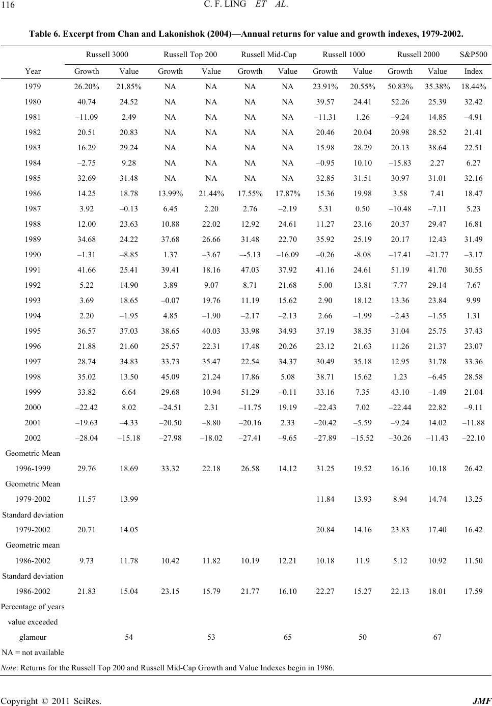
Indeed, in Table 6 we can see that in 2000, the Russell
Top 200 Growth Index fell by 24.51%, followed by a
decline of 20.5% the next year. On the other hand, the
Russell 2000 Value Index rose by 22.82% and 14.02%,
respectively. This indicates that investors finally realized
that those “growth” companies had fallen short of their
expec tations, and a pr ice adjustmen t occurred as a result.
Looking at the overall record, from 1979 to 2002, the geo-
metric return of value stocks still outperformed growth
stocks. From Table 6, it was 13.99% vs. 11 .57% for large-
cap stocks, and 14.74% vs. 8.94% for small-cap stocks.
There were some discrepancies in the Russell index,
however, as it did not represent extreme bets on growth
or value since only two portfolios were formed (instead
of 10). Further, the underlying stocks were value weighted
and rely on only two indicators (BV/MV and analysts’
long-term growth forecasts). To address this concern,
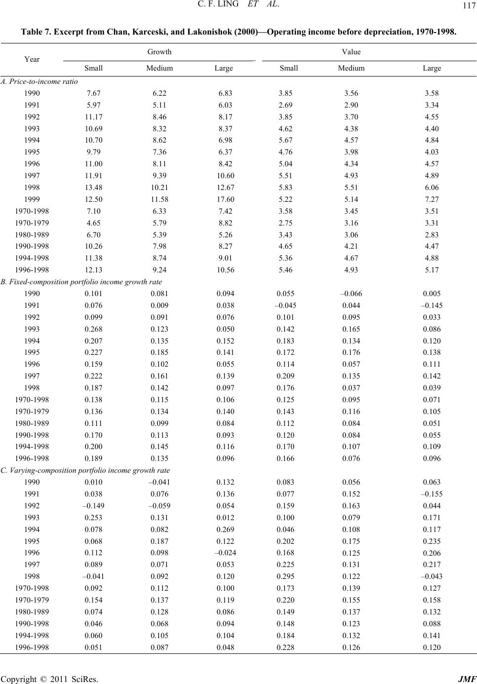
Chan and Lakonishok [8] performed another analysis by
sorting stocks using a composite indicator and placing
them in 10 deciles with each stocks equally weighted in
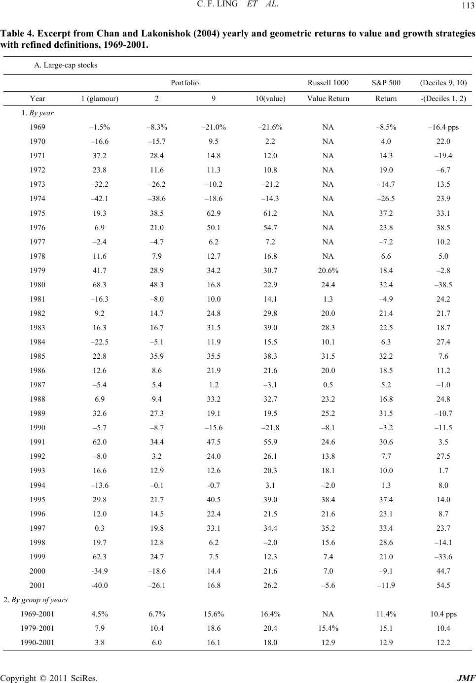
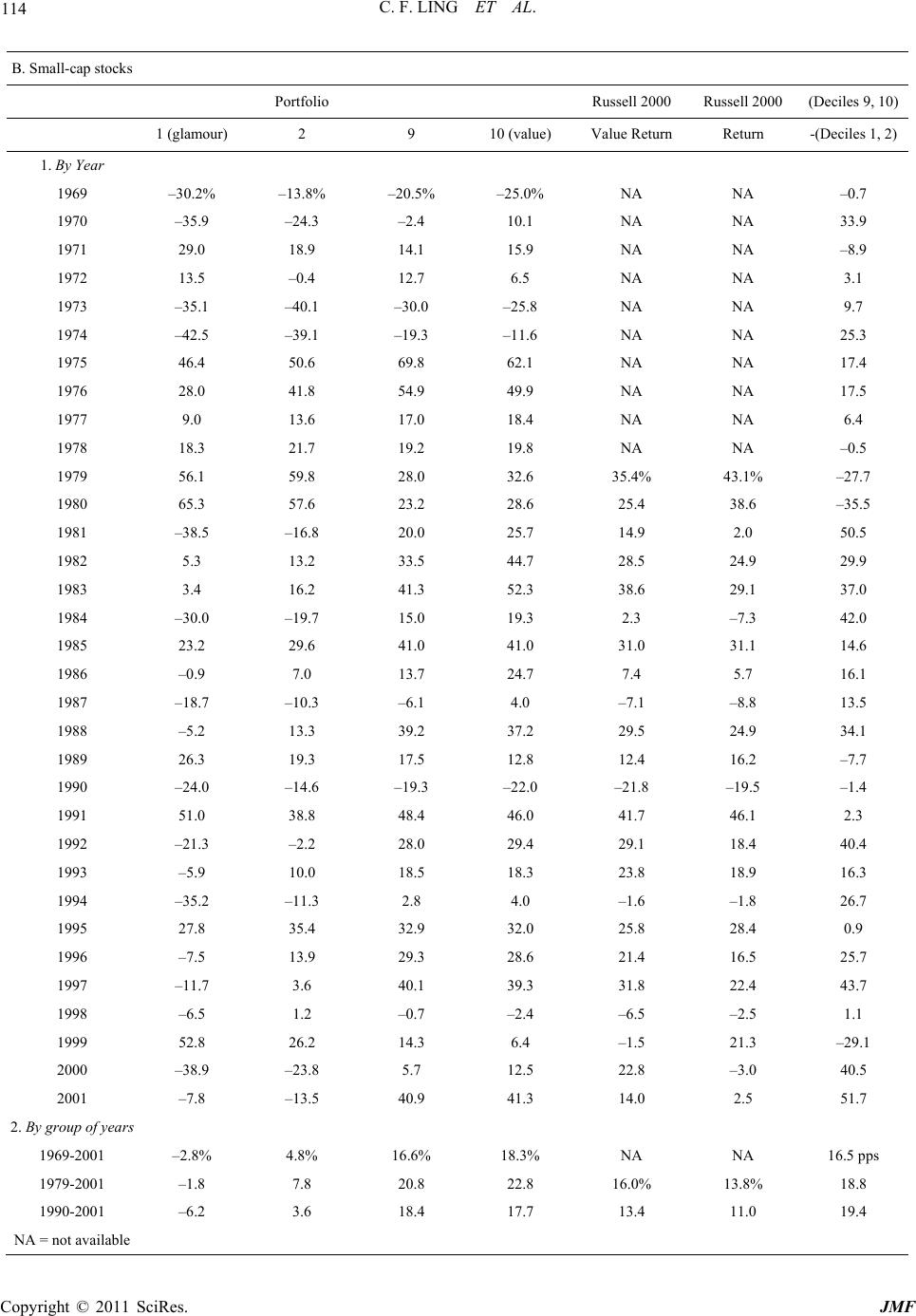
each portfolio. The results are shown in Table 4. From
1996-2001, we can see that for large-cap stocks (Panel
A), the value portfolio only fell behind the growth port-
folio in 1998 and 1999, and cau ght up again in 2000 and
2001. As a result, the geometric return for value stocks
from 1990-2001 is 16.1%, compared to 3.8% for growth
stocks. For small cap stocks, the spread is even more sig-
nificant: 18.4% for value compared to –6.2% for growth.
3. Conclusions
Various studies provided evidence that value stocks could
generate superior return than growth stocks. This spread
is often more significant in the small-cap stocks than in
the large-cap stocks, indicating that part of the spread must
be attributed to size of the companies. In addition, the
studies showed that systematic risk cannot not be accounted
for the spread as both glamour and value portfolios have
similar beta.
Further studies showed that even we took the compa-
nies’ size into account, the spread still existed. This leads
to the assertion there is a value premium that con tributes
to the spread. The reasons of the existence of value pre-
mium will be explored later. But in a vague sense, some
scholars argued that this could be caused by extrapola-
tion bias: people incorrectly use past data to predict fu-
ture performance of a company.
In addition, a number of different indicators could be
used to yield value premium. And a combination of such
indicators could often yield a higher return than using
just a single indicator.
On the other hand, the persisting superior return of
growth stocks in late 1990s seemed to invalidate the claim
of value premium. However, further study showed that
those “growth” companies didn’t realize any stronger
subsequent earnings growth than value companies even
though their P/I ratio continued to be high. There was
also a rigorous price adjustment in late 2000 and 2001,
with value stocks skyrocketing and growth stocks plum-
meting. Combining these two pieces of evidence, some
scholars argued that the value premium did not disappear.
Instead, it just took longer for the price reversion to oc-
cur as market persisted to have rosy expectation to tech-
nology companies.
4. References
[1] B. Graham and D. Dodd, “Security Analysis,” 6th Edition,
Graw-Hill, New York City, 2009, pp. 61-70.
[2] S. Basu, “Investment Performance of Common Stocks in
Relation to Their Price-Earnings Ratios: A Test of the Ef-
ficient Market Hypothesis,” Journal of Finance, Vol. 32,
No. 3, 1977, pp. 255-274. doi:10.2307/2326304
[3] E. F. Fama and K. R. French, “The Cross-Section of Ex-
pected Stock Returns,” Journal of Finance, Vol. 47, No.
2, 1992, pp. 427-465. doi:10.2307/2329112
[4] J. Lakonishok, A. Shleifer and R. W. Vishny, “Contrarian
Investment, Extrapolation, and Risk,” Journal of Finance,
Vol. 49, No. 5, 1994, pp. 1541-1578.
doi:10.2307/2329262
[5] L. K. C. Chan, Y. Hamao, and J. Lakonishok, “Funda-
mentals of Stock Return in Japan,” Journal of Finance,
Vol. 46, No. 5, 1991, pp. 1739-1764.
doi:10.2307/2328571
[6] E. F. Fama and K. R. French. “Value versus Growth: The
International Evidence,” Journal of Finance, Vol. 53, No.
6, 1998, pp. 1975-1999. doi:10.1111/0022-1082.00080
[7] R. W. Banz, “The Relationship between Return and
Market Value of Common Stock,” Journal of Financial
Economics, Vol. 9, No. 1, 1981, pp. 3-18.
doi:10.1016/0304-405X(81)90018-0
[8] L. K. C. Chan and J. Lakonishok, “Value and Growth
Investing: Review and Update,” Financial Analyst Jour-
nal, Vol. 60, No. 1, 2004, pp. 71-86.
doi:10.2469/faj.v60.n1.2593
[9] C. Asness, “The Interaction of Value and Momentum
Strategies,” Financial Analysts Journal, Vol. 53, No. 2
1997, pp. 29-36. doi:10.2469/faj.v53.n2.2069
[10] D. Kent and S. Titman, “Market Efficiency in an Irra-
tional World,” Financial Analysts Journal, Vol. 55, No. 6
1999, pp. 28-40. doi:10.2469/faj.v55.n6.2312

119 C. F. LING ET AL.
[11] L. K. C. Chan, J. Lakonishok and T. Sougiannis, “The
Stock Market Valuation of Research and Development
Expenditures,” Journal of Finance, Vol. 56, No. 6, 2001.
pp. 2431-2456. doi:10.1111/0022-1082.00411
[12] J. Piotroski, “Value Investing: The Use of Historical Fi-
nancial Statement Information to Separate Winners from
Losers,” Journal of Accounting Research, Vol. 38, 2000,
pp. 1-41. doi:10.2307/2672906
[13] L. K. C. Chan, J. Karceski and J. Lakonishok, “New
Paradigm or Same Old Hype in Equity Investing?” Fi-
nancial Analysts Journal, Vol. 56, No. 4, 2000, pp. 23-36.
doi:10.2469/faj.v56.n4.2371