 Journal of Mathematical Finance, 2011, 1, 41-49 doi:10.4236/jmf.2011.13006 Published Online November 2011 (http://www.SciRP.org/journal/jmf) Copyright © 2011 SciRes. JMF Adaptive Wave Models for Sophisticated Option Pricing Vladimir G. Ivancevic Defence Science & Technology Organisation, Canberra, Australia E-mail: Vladimir.Ivancevic@dsto.defence.gov.au Received August 19, 2011; revised October 13, 2011; accepted October 22, 2011 Abstract Adaptive wave model for financial option pricing is proposed, as a high-complexity alternative to the stan- dard Black-Scholes model. The new option-pricing model, representing a controlled Brownian motion, in- cludes two wave-type approaches: nonlinear and quantum, both based on (adaptive form of) the Schrödinger equation. The nonlinear approach comes in two flavors: for the case of constant volatility, it is defined by a single adaptive nonlinear Schrödinger (NLS) equation, while for the case of stochastic volatility, it is de- fined by an adaptive Manakov system of two coupled NLS equations. The linear quantum approach is de- fined in terms of de Broglie’s plane waves and free-particle Schrödinger equation. In this approach, financial variables have quantum-mechanical interpretation and satisfy the Heisenberg-type uncertainty relations. Both models are capable of successful fitting of the Black-Scholes data, as well as defining Greeks. Keywords: Black-Scholes Option Pricing, Adaptive Nonlinear Schrödinger Equation, Adaptive Manakov System, Quantum-Mechanical Option Pricing, Market-Heat Potential 1. Introduction Recall that the celebrated Black-Scholes partial differ- ential equation (PDE) describes the time-evolution of the market value of a stock option [1,2]. Formally, for a function defined on the domain =,uuts , 00< tT and describing the market value of a stock option with the stock (asset) price , the Black- Scholes PDE can be written (using the physicist notation: = zuuz) as a diffusion-type equation: 2 1 = 2 tsss usursu ,ru (1) where >0 is the standard deviation, or volatility of s, r is the short-term prevailing continuously—compounded risk—free interest rate, and is the time to matur- ity of the stock option. In this formulation it is assumed that the underlying (typically the stock) follows a geomet- ric Brownian motion with “drift” >0T and volatility , given by the stochastic differential equation (SDE) [3] d= dd , tsttstWt (2) where W is the standard Wiener process. The Black-Scholes PDE (1) is usually derived from SDEs describing the geometric Brownian motion (2), with the stock-price solution given by: 12 2 =0etWt st s . In mathematical finance, derivation is usually perfor- med using Itô lemma [4] (assuming that the underlying asset obeys the Itô SDE), while in physics it is performed using Stratonovich interpretation [5,6] (assuming that the underlying asset obeys the Stratonovich SDE [8]). The Black-Sholes PDE (1) can be applied to a number of one-dimensional models of interpretations of prices given to u, e.g., puts or calls, and to s, e.g., stocks or fu- tures, dividends, etc. The most important examples are European call and put options, defined by: Call 12 ,=dede , T usts k rT (3) Put2 1 ,=dede , rT T ustks (4) 1 ()=1 erf, 22 2 1 ln 2 d= , sTr k T 2 2 ln 2 d= , sTr k T  42 V. G. IVANCEVIC where erf is the (real-valued) error function, k de- notes the strike price and represents the dividend yield. In addition, for each of the call and put options, there are five Greeks (see, e.g. [9,10]), or sensitivities, which are partial derivatives of the option-price with respect to stock price (Delta), interest rate (Rho), volatility (Vega), elapsed time since entering into the option (Theta), and the sec- ond partial derivative of the option-price with respect to the stock price (Gamma). Using the standard Kolmogorov probability approach, instead of the market value of an option given by the Black-Scholes Equation (1), we could consider the cor- responding probability density function (PDF) given by the backward Fokker-Planck equation (see [6,7]). Al- ternatively, we can obtain the same PDF (for the market value of a stock option), using the quantum-probability formalism [11,12], as a solution to a time-dependent linear or nonlinear Schrödinger equation for the evolution of the complex-valued wave -function for which the absolute square, 2, is the PDF. The adaptive nonlin- ear Schrödinger (NLS) equation was recently used in [10] as an approach to option price modelling, as briefly re- viewed in this section. The new model, philosophically founded on adaptive markets hypothesis [13,14] and Elliott wave market theory [15,16], as well as my own recent work on quantum congition [17,18], describes adaptively controlled Brownian market behavior. This nonlinear ap- proach to option price modelling is reviewed in the next section. Its important limiting case with low interest-rate reduces to the linear Schrödinger equation. This linear approach to option price modelling is elaborated in the subsequent section. 2. Nonlinear Adaptive Wave Model for General Option Pricing 2.1. Adaptive NLS Model The adaptive, wave-form, nonlinear and stochastic option- pricing model with stock price s, volatility and interest rate r is formally defined as a complex-valued, focusing (1+1)-NLS equation, defining the time-dependent op- tion-price wave function =, t , whose absolute square 2 , t represents the probability density func- tion (PDF) for the option price in terms of the stock price and time. In natural quantum units, this NLS equation reads: 2 1 =,= 2 tss ii 1, m (5) where denotes the adaptive market-heat po- tential (see [19]), so the ter =,rw 2 =V the represents -dependent potential field. In the simplest nonadap- tive scenario is equal to the interest rate r, while in the adaptive case it depends on the set of adjustable syn- aptic weights i w as: 2 1 =1 3 ,= erf i nii i ws .r ww rw (6) Physically, the NLS Equation (5) describes a nonlinear wave (e.g. in Bose-Einstein condensates) defined by the complex-valued wave function , t of real space and time parameters. In the present context, the space-like variable s denotes the stock (asset) price. The NLS Equation (5) has been exactly solved using the power series expansion method [20,21] of Jacobi elliptic functions [22]. Consider the -function descri- bing a single plane wave, with the wave number k and circular frequency : i ,=e , ks t st (7) with =andskt . Its substitution into the NLS Equation (5) gives the nonlinear oscillator ODE: 23 1=0. 2 '' k (8) We can seek a solution for (8) as a linear func- tion [21] 01 =snaa , where sn,= sn sm are Jacobi elliptic sine func- tions with elliptic modulus 0,1m, such that sn= sin,0 sand sn,1= tanh s. The solution of (8) was calculated in [10] to be = sn,for 0,1, mm =tanh,for =1.m This gives the exact periodic solution of (5) as [10] 0,1 m 22 1 i1 2 ,=sn e, kstm k sts kt w m 1 for ; (9) 2 1 i2 2 2 for ,= 1, tanh e, = kst k sts kt w m (10) where (9) defines the general solution, while (10) defines C opyright © 2011 SciRes. JMF 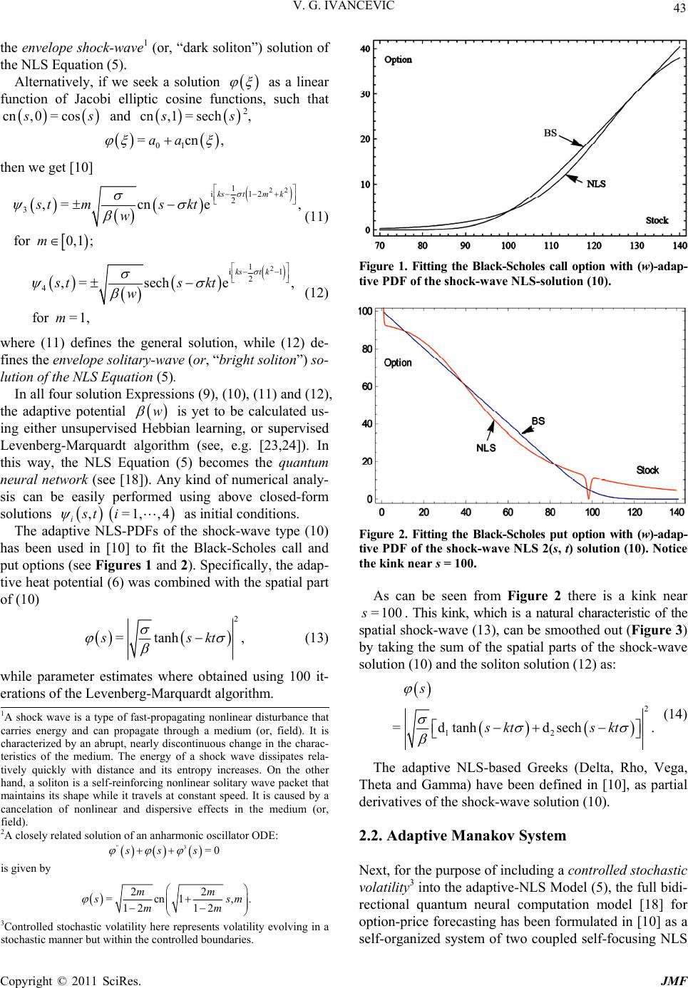 43 V. G. IVANCEVIC the envelope shock-wave1 (or, “dark soliton”) solution of the NLS Equation (5). Alternatively, if we seek a solution as a linear function of Jacobi elliptic cosine functions, such that cn,0= cos s and cn ,1= sech s2, 01 =cnaa , then we get [10] 22 1 i12 2 3,=cn e, for 0,1; kstmk stms kt w m (11) 2 1 i1 2 4, =seche, for =1, kst k sts kt w m (12) where (11) defines the general solution, while (12) de- fines the envelope solitary-wave (or, “bright soliton”) so- lution of the NLS Equation (5). In all four solution Expressions (9), (10), (11) and (12), the adaptive potential is yet to be calculated us- ing either unsupervised Hebbian learning, or supervised Levenberg-Marquardt algorithm (see, e.g. [23,24]). In this way, the NLS Equation (5) becomes the quantum neural network (see [18]). Any kind of numerical analy- sis can be easily performed using above closed-form solutions as initial conditions. w =1, ,4 , st i i The adaptive NLS-PDFs of the shock-wave type (10) has been used in [10] to fit the Black-Scholes call and put options (see Figures 1 and 2). Specifically, the adap- tive heat potential (6) was combined with the spatial part of (10) 2 =tanhssk ,t (13) while parameter estimates where obtained using 100 it- erations of the Levenberg-Marquardt algorithm. Figure 1. Fitting the Black-Scholes call option with (w)- adap- tive PDF of the shock-wave NLS-solution (10). Figure 2. Fitting the Black-Scholes put option with (w)- adap- tive PDF of the shock-wave NLS 2(s, t) solution (10). Notice the kink near s = 100. As can be seen from Figure 2 there is a kink near . This kink, which is a natural characteristic of the spatial shock-wave (13), can be smoothed out (Figure 3) by taking the sum of the spatial parts of the shock-wave solution (10) and the soliton solution (12) as: = 100s 2 12 =d tanhd sech. s skt skt (14) 1A shock wave is a type of fast-propagating nonlinear disturbance that carries energy and can propagate through a medium (or, field). It is characterized by an abrupt, nearly discontinuous change in the charac- teristics of the medium. The energy of a shock wave dissipates rela- tively quickly with distance and its entropy increases. On the other hand, a soliton is a self-reinforcing nonlinear solitary wave packet that maintains its shape while it travels at constant speed. It is caused by a cancelation of nonlinear and dispersive effects in the medium (or, field). 2A closely related solution of an anharmonic oscillator ODE: 3=0 '' ss s is given by 22 =cn1 , 12 12 mm The adaptive NLS-based Greeks (Delta, Rho, Vega, Theta and Gamma) have been defined in [10], as partial derivatives of the shock-wave solution (10). 2.2. Adaptive Manakov System Next, for the purpose of including a controlled stochastic volatility3 into the adaptive-NLS Model (5), the full bidi- rectional quantum neural computation model [18] for option-price forecasting has been formulated in [10] as a self-organized system of two coupled self-focusing NLS . sm mm 3Controlled stochastic volatility here represents volatility evolving in a stochastic manner but within the controlled boundaries. Copyright © 2011 SciRes. JMF 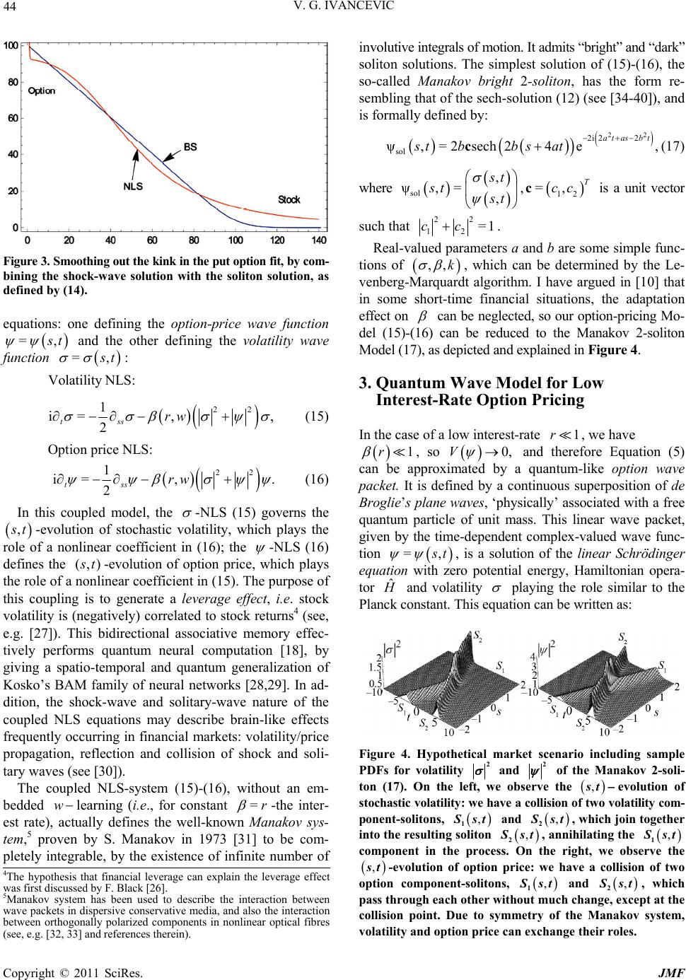 44 V. G. IVANCEVIC Figure 3. Smoothing out the kink in the put option fi t, by com- bining the shock-wave solution with the soliton solution, as defined by (14). equations: one defining the option-price wave function =, t and the other defining the volatility wave function =, t : Volatility NLS: 22 1 i= , 2 tss rw , (15) Option price NLS: 22 i= , . 2 tss rw 1 (16) In this coupled model, the -NLS (15) governs the , t-evolution of stochastic volatility, which plays the role of a nonlinear coefficient in (16); the -NLS (16) defines the (,) t-evolution of option price, which plays the role of a nonlinear coefficient in (15). The purpose of this coupling is to generate a leverage effect, i.e. stock volatility is (negatively) correlated to stock returns4 (see, e.g. [27]). This bidirectional associative memory effec- tively performs quantum neural computation [18], by giving a spatio-temporal and quantum generalization of Kosko’s BAM family of neural networks [28,29]. In ad- dition, the shock-wave and solitary-wave nature of the coupled NLS equations may describe brain-like effects frequently occurring in financial markets: volatility/price propagation, reflection and collision of shock and soli- tary waves (see [30]). The coupled NLS-system (15)-(16), without an em- bedded learning (i.e., for constant w=r -the inter- est rate), actually defines the well-known Manakov sys- tem,5 proven by S. Manakov in 1973 [31] to be com- pletely integrable, by the existence of infinite number of involutive integrals of motion. It admits “bright” and “dark” soliton solutions. The simplest solution of (15)-(16), the so-called Manakov bright 2-soliton, has the form re- sembling that of the sech-solution (12) (see [34-40]), and is formally defined by: 22 2i 22 sol ψ,= 2sech24e, atasbt stbb satc(17) where sol , ψ,= , t st t, is a unit vector such that 12 =,T ccc 22 12 =1cc. Real-valued parameters a and b are some simple func- tions of ,,k , which can be determined by the Le- venberg-Marquardt algorithm. I have argued in [10] that in some short-time financial situations, the adaptation effect on can be neglected, so our option-pricing Mo- del (15)-(16) can be reduced to the Manakov 2-soliton Model (17), as depicted and explained in Figure 4. 3. Quantum Wave Model for Low Interest-Rate Option Pricing In the case of a low interest-rate , we have 1r 1r , so 0,V and therefore Equation (5) can be approximated by a quantum-like option wave packet. It is defined by a continuous superposition of de Broglie’s plane waves, ‘physically’ associated with a free quantum particle of unit mass. This linear wave packet, given by the time-dependent complex-valued wave func- tion ,= t ˆ , is a solution of the linear Schrödinger equation with zero potential energy, Hamiltonian opera- tor and volatility playing the role similar to the Planck constant. This equation can be written as: Figure 4. Hypothetical market scenario including sample PDFs for volatility 2 and 2 of the Manakov 2-soli- ton (17). On the left, we observe the evolution of stochastic volati lity: we have a collision of two volatility com- ponent-solitons, ,st , 1 st and , 2 st , which join together into the resulting soliton , 2 st , annihilating the , 1 st component in the process. On the right, we observe the ,st -evolution of option price: we have a collision of two option component-solitons, , 1 st and , 2 st , which pass through each other without much change, except at the collision point. Due to symmetry of the Manakov system, volatility and option price can exchange their roles. 4The hypothesis that financial leverage can explain the leverage effect was first discussed by F. Black [26]. 5Manakov system has been used to describe the interaction between wave packets in dispersive conservative media, and also the interaction between orthogonally polarized components in nonlinear optical fibres see, e. . 32, 33 and references therein . C opyright © 2011 SciRes. JMF  45 V. G. IVANCEVIC 2 ˆˆ i=,where= 2 ts HH . s (18) Thus, we consider the -function describing a single de Broglie’s plane wave, with the wave number k, linear momentum =pk, wavelength =2π, kk angular frequency 2 =2, kk and oscillation period 2 =4=2T kkk . It is defined by (compare with [41,42,12]) 2 i2 i 22 ,=e =e =cosisin , 2 k k ks t ks t kst AA kk 2 kstAkst (19) where A is the amplitude of the wave, the angle 2 =2 kk ks tkst represents the phase of the wave k with the phase velocity: == kk vkk2. The space-time wave function , t that satisfies the lin- ear Schrödinger Equation (18) can be decomposed (using Fourier’s separation of variables) into the spatial part and the temporal part i et as: i i ,=e=e. t t st ss The spatial part, representing stationary (or, amplitude) wave function, satisfies the linear har- monic oscillator, which can be formulated in several equivalent forms: i =e, ks sA 2 2 2 2 =0, =0, 2 =0, =0. '' '' '' '' kk k p k E v (20) Planck’s energy quantum of the option wave k is given by: 2 1 == 2 kk Ek . From the plane-wave expressions (19) we have: i ,=e sEt k kst A —for the wave going to the “right” and i ,=e sEt k kst A —for the wave going to the “left”. The general solution to (18) is formulated as a linear combination of de Broglie’s option waves (19), compris- ing the option wave-packet: =0 ,=, , (with). n ik i i stc stn (21) Its absolute square, 2 ,, t represents ability density function at a time t. n option by the prob- The group velocity of a wave-packet is given : =dd . gk vk It is related to the phase velocity v of a plane wave as: k =dd. kkkk vv v Closely related is the center of the option wave-pack t (the point of maximu e m amplitude), given: by =d d. k tk The following quantum-motivated assertions can be stated: y 1) Volatilit has dimension of financial action, or energy time. 2) The total rgy E of an option wave-packet is (in the case of simil r plane waves) given by Planck’s su- perposition of the ene a energies k E of n individual waves: 2 == , 2 kn En k =Ln where denotes the angular momentum of the option wave-packet, representing the shift between its and decaygrowth, and vice versa. 3) The average energy E of an option wave-packet is given by Boltzmann’s partition function: =0 e ==, k T k nk nE E E =0 ee 1 b nE E kk bT bT n where b is the Boltzmann-like kinetic constant and T is the market temperature. nE 4) The energy form of the Schrödinger Equation (18) reads: =i t E . 5) The eigenvalue equation for the Hamiltonian op- erator ˆ is the stationary Schr ödi nger equation: 2 ˆ=,or =, 2ss sEs Ess which is just another form of the harmonic oscillator (20). It has oscillatory solutions of the form: ii 22 12 =ee, sEs kk Esc c called energy eigen-states with energies and deno- ted by: k E EkE ˆ=. sE s The Black-Scholes put and call options have been fit- ted with the quantum PDFs (see Figures 5 and 6) given by t opti the absolute square of (21) with =7n and =3n, respectively. Using supervised Levenberg-Marquardt al- gorithm and Mathematica 7, the following coefficients were obtained for the Black-Scholes puon: Copyright © 2011 SciRes. JMF  46 V. G. IVANCEVIC Figure 5. Fitting the Black-Scholes put option with the quan- tum PDF given by the absolute square of (21) with n = 7. Figure 6. Fitting the Black-Scholes call option with the quan- tum PDF given by the absolute square of (21) with n = 3. Note that fit is good in the realistic stock region: Using the same algorithm, the following coefficients were obtained for the Black-Scholes call option: Now, given some initial option wave function, []75,140s. ** =0.0031891, =0.0031891, =2.62771, =2.62777, =2.65402, t kkk 123 4567 12 345 67 =2.61118, =2.64104, =2.54737, =2.62778, =1.26632, =1.26517, =2.74379, =1.35495, =1.59586, =0.263832, =1.26779, with kk cc ccc cc ** =94.0705, =31.3568. BS BS tt kk ** 12 31 23 ** =11.9245, =11.9245, =0.851858, =0.832409, =0.872061, =2.9004, =2.72592, =2.93291, with0.0251583, =0.00838609. BS t kk kc cc tt ,0 =, 0 s a solution to the initial-value problem for the linear Schrö- dinger Equation (18) is, in terms of the pair of Fourier transforms 1 ,, given by (see [42]) 2 i 1i12 00 ,st =e =e. kt t (22) p- tion wave-function at time t = 0 givby the complex- valued Gaussian function: he width p is the av- erage momentum of the wave. Its Fourier transform, For example (see [42]), suppose we have an initial o en 2/2 i ,0=ee, as ks s where a is tof the Gaussian, while 0 ˆ=,0ks , is given by 2 2 0 e ˆ=. kp a ka The solution at time t of the initial value problem is given by 22 i22 1 ,=ee d, 2π kk p ks ta a tk a which, after some algebra becomes 22 2i i exp 21 i ,=,with =. 1i asspp t at tp at k iven by the real-valued Gaussian function, As a simpler example,6 if we have an initial option wave- function g 22 4 e ,0 =, s s the solution of complex-valued (18) is given by the - function, 2 4 exp 21 i ,= . 1i s t st t 6An example of a more general Gaussian wave-packet solution of (18) is given by: 22 0000 1i i 22 ,= exp, 1i1i as sptpss a st at at where 00 , p t are initial stock-price and average momentum, while ais the width of the Gaussian. At time the `particle' is at rest around , its average momentum 0. The wave function spreads with time while its maximum decreases and stays put at the origin. At time the wave packet is the complex-conjugate of the wave-packet at time t. =0t =0p =0s C opyright © 2011 SciRes. JMF  47 V. G. IVANCEVIC From (22) it follows that a stationary option wave-packet is given by: i 1ˆˆ =ed,where=[ 2 ks ]. kkk s As 2 is the stationary stock PDF, we can cal- culate the expectation values of the stock and the wave number of the whole option wave-packet, consisting of n measured plane waves, as: 2 ˆ =dand= 2 d. ss skk kk (23) red around the mean values (23). The width of the distribution of the recorded The recordings of n individual option plane waves (19) will be scatte - and -values are uncertainties k and respectively. The satisfy th Heisenberg-type uncertainty relation: ,k ye , 2 n sk which imply the similar relation for the total option en- ergy and time: . 2 4. A New Stock-Market Research Program Based on the above wave stock-market a n Et nalysis, I pro- pose a new financial research program as follows. Firstly, define the general adaptive wave model for option pricing evolution as a (linear) combination of the (5). The three wave-components of this general model are: 1) the linear wave packet previously defined particular solutions to the adaptive NLS-Equation pack , et t , given by (21); 2) the shock-wave , shock t , given by (10); and 3) the soliton soliton , t , given by (12). Formally, the general adaptive wave model is defined by: 21 2 3sec , ks t k As 2 i general 1 =0 1 i2 2 2 ,= e tanhe k ks t i i kst k stA c Askt 1 i h e kt w dentudes of the t in Secondly, we need to find the most representative fi- nancial index or contemporary markets data that clearly show in their evolution both the efficient markets hy- pothesis [13] and adaptive markets hypothesis [14]. Once we find such a representative data, we need to fit it using our general wave Model (24) and the powerful Len- berg-Marquardt fitting algorithm. I remark here that, based on my empirical experience, the general wave Model (24) is capable of fitting any financial data, provided we use appropriate number of fitting coefficients (see [10] for al details). l have a model that can be used fo waves. For the purpose of fitting a, the Levenberg-Marquardt algo- n here , =1, i Ai ote adaptive ampli, 5 hree waves, while the other parameters are defined the previous section. ve technic Once we have successfully fitted the most representa- tive market data we wil r prediction of many possible outcomes of the current global financial storm. 5. Conclusions I have proposed an adaptive-wave alternative to the stan- dard Black-Scholes option pricing model. The new model, philosophically founded on adaptive markets hypothesis [13,14] and Elliott wave market theory [15,16], describes adaptively controlled Brownian market behavior. Two ap- proaches have been proposed: 1) a nonlinear one based on the adaptive NLS (solved by means of Jacobi elliptic functions) and the adaptive Manakov system (of two coupled NLS equations); 2) a linear quantum-mecha- nical one based on the free-particle Schrödinger equation nd de Broglie’s plane a the Black-Scholes dat rithm was used. The presented adaptive and quantum wave models are spatio-temporal dynamical systems of much higher com- plexity [25] then the Black-Scholes model. This makes the new wave models harder to analyze, but at the same time, their immense variety is potentially much closer to the real financial market complexity, especially at the time of financial crisis. 6. References [1] F. Black and M. Scholes, “The Pricing of Options and Corporate Liabilities,” Journal of Political Economy, Vol. 81, No. 3, 1973, pp. 637-659. doi:10.1086/260062 [2] R. C. Merton, “Theory of Rational Option Pricing,” The Bell Journal of Economics and Management Science, Vol. 4, No. 1, 1973, pp. 141-183. doi:10.2307/3003143 [3] M. F. M. Osborne, “Brownian Motion in the Stock Mar- ket,” Operations Research, Vol. 7, No. 2, 1959, pp. 145- 173. doi:10.1287/opre.7.2.145 [4] K. Itô, “On Stochastic Differential Equations,” Memoirs of the American Mathematical Society, Vol. 4, 1951, pp. 1-51. M. Porra, M. Montero and J. Masoliver, Black-Scholes Option Pricing within Itô and Stratonovich Conventions, Physica A: Statistical Mechanics and Its [5] J. Perello, J. Copyright © 2011 SciRes. JMF  48 V. G. IVANCEVIC Applications, Vol. 278, No. 1-2, 2000, pp. 260-274. doi:10.1016/S0378-4371(99)00612-3 [6] C. W. Gardiner, “Handbook of Stochastic Methods,” Sprin- 6, pp. 362-371. ger, Berlin, 1983. [7] J. Voit, “The Statistical Mechanics of Financial Markets,” Springer, Berlin, 2005. [8] R. L. Stratonovich, “A New Representation for Stochastic Integrals and Equations,” SIAM Journal on Control and Optimization, Vol. 4, No. 2, 196 doi:10.1137/0304028 [9] M. Kelly, “Black-Scholes Option Model & European Op- tion Greeks,” The Wolfram Demonstrations Project, 2009 ynamics in Complex Variables,” Sprin- ancevic, “Quantum Leap: From . http://demonstrations.wolfram.com/EuropeanOptionGree ks [10] V. Ivancevic, “Adaptive-Wave Alternative for the Black- Scholes Option Pricing Model,” Cognitive Computat Vol. 2, No. 1, 2010, pp. 17-30. ion, [11] V. Ivancevic and T. Ivancevic, “Complex Dynamics: Ad- vanced System D ger, Dordrecht, 2007. [12] V. Ivancevic and T. Iv Dirac and Feynman, Across the Universe, to Human Body and Mind,” World Scientific, Singapore, 2008. doi:10.1142/9789812819284 [13] A. W. Lo and J. Portf, “The Adaptive Markets Hypothe- sis: Market Efficiency from an Evolutionary Perspec- tive,” Journal of Portfolio Management, Vol. 30, 2004, pp. 15-29. A. [14] W. Lo and J. Inves, “Reconciling Efficient Markets with Behavioral Finance: The Adaptive Markets Hy- pothesis,” Journal of Investment Consulting, Vol. 7, 2005, pp. 21-44. [15] A. J. Frost and R. R. Prechter Jr., “Elliott Wave Principle: Key to Market Behavior,” 10th Edition, Wiley, New York, 1978. [16] P. Steven, “Applying Elliott Wave Theory Profitably,” Wi- ley, New York, 2003. [17] V. Ivancevic and E. Aidman, “Life-Space Foam: A Me- dium for Motivational and Cognitive Dynamics,” Physica A: Statistical Me chanics and its A pplications, Vol. 382, No. 2, 2007, pp. 616-630. doi:10.1016/j.physa.2007.04.025 [18] V. Ivancevic and T. Ivancevic, “Quantum Neural Com- putation,” Springer, Berlin, 2009. [19] H. Kleinert and H. Kleinert, “Path Integrals in Quantum Mechanics, Statistics, Polymer Physics, and Financial Markets,” 3rd Edition, World Scientific, Singapore, 2002. [20] S. Liu, Z. Fu, S. Liu and Q. Zhao, “Jacobi Elliptic Function Expansion Method and Periodic Wave Solutions of Non- linear Wave Equations,” Physics Letters A, Vol. 289, No. 1-2, 2001, pp. 69-74. doi:10.1016/S0375-9601(01)00580-1 [21] G.-T. Liu and T.-Y. Fan, “New Applications of Devel- oped Jacobi Elliptic Function Expansion Methods,” Phy- sics Letters A, Vol. 345, No. 1-3, 2005, pp. 161-166. doi:10.1016/j.physleta.2005.07.034 [22] M. Abramowitz and I. A. Stegun, Eds., “Jacobian Elliptic Functions and Theta Functions. Chapter 16 in Handbook of Mathematical Functions with Formulas, Graphs, and Mathematical Tables,” 9th Edition, Dover, New York, 1972, pp. 567-581. [23] V. Ivancevic and T. Ivancevic,” Neuro-Fuzzy Associative Machinery for Comprehensive Brain and Cognition Mo- delling,” Springer, Berlin, 2007. doi:10.1007/978-3-540-48396-0 [24] V. Ivancevic and T. Ivancevic, “Computational Mind: A Complex Dynamics Perspective,” Springer, Berlin, 2007. doi:10.1007/978-3-540-71561-0 [25] V. Ivancevic and T. Ivancevic, “Complex Nonlinearity: Chaos, Phase Transitions, Topology Change and Path In- tegrals,” Springer, Berlin, 2008. [26] F. Black, “Studies of Stock Price Volatility Changes,” Proceedings of the 1976 Meetings of the American Statis- tical Association, Business and Economics Statistics Sec- tion, 1976, pp. 177-181. [27] H. E. Roman, M. Porto and C. Dose, “Skewness, Long- Time Memory, and Nonstationarity: Application to Lev- erage Effect in Financial Time Series,” Europhysics Let- ters, Vol. 84, No. 2, 2008, pp. 28001-28006. [28] B. Kosko, “Bidirectional Associative Memories,” IEEE Transactions on Systems, Man and Cybernetics, Vol. 18, No. 1, 1988, pp. 49-60. doi:10.1109/21.87054 [29] B. Kosko, “Neural Networks, Fuzzy Systems, A Dynami- cal Systems Approach to Machine Intelligence,” Pren- tice Hall, Upper Saddle River, 1992. [30] S.-H. Hanm, I. G. Koh, “Stability of Neural Networks and Solitons of Field Theory,” Physical Review E, Vol. 60, No. 6, 1999, pp. 7608-7611. doi:10.1103/PhysRevE.60.7608 [31] S. V. Manakov, “On the Theory of Two-Dimensional in Isotropic Stationary Self-Focusing of Electromagnetic Waves,” Soviet Physics JETP, Vol. 38, p. 248. [32] M. Haelterman and A. P. Sheppard, “Bifurcation Phe- nomena and Multiple Soliton-Bound States Kerr Media,” Physical Review E, Vol. 49, No. 4, 1994, pp. 3376-3381. doi:10.1103/PhysRevE.49.3376 [33] J. Yang, “Classification of the Solitary Waves in Coupled Nonlinear Schrödinger Equations,” Physica D: Nonlinear Phenomena, Vol. 108, No. 1-2, 1997, pp. 92-112. doi:10.1016/S0167-2789(97)82007-6 [34] D. J. Benney and A. C. Newell, “The propagation of Nonlinear Wave Envelops,” Journal of Mathematical Physics, Vol. 46, 1967, pp. 133-139. [35] V. E. Zakharov, S. V. Manakov, S. P. Novikov and L. P. olitons in Optical E, Vol. 56, Pitaevskii, “Soliton Theory: Inverse Scattering Method. Nauka, Moscow, 1980. [36] A. Hasegawa and Y. Kodama, “S Communications,” Clarendon, Oxford, 1995. [37] R. Radhakrishnan, M. Lakshmanan and J. Hietarinta, “Inelastic Collision and Switching of Coupled Bright Solitons in Optical Fibers,” Physical Review No. 2, 1997, pp. 2213-2216. C opyright © 2011 SciRes. JMF  V. G. IVANCEVIC Copyright © 2011 SciRes. JMF 49 doi:10.1103/PhysRevE.56.2213 [38] G. Agrawal, “Nonlinear Fiber Optics,” 3rd Edition, Aca- demic Press, San Diego, 2001. J. Yang, “Interactions of Vector Solit[39] ons,” Physical Re- view E, Vol. 64, No. 2, 2001, pp. 026607-026623. doi:10.1103/PhysRevE.64.026607 [40] J. Elgin, V. Enolski and A. Its, “Effective Integration of the Nonlinear Vector Schrödin Nonlinear Phenomena, Vol. 225, No. 2 ger Equation,” Physica D: , 2007, pp. 127- 152. doi:10.1016/j.physd.2006.10.005 [41] D. J. Griffiths, “Introduction to Quantum Mechanics,’ New 2nd Edition, Pearson Educ. Int., (2005) [42] B. Thaller, “Visual Quantum Mechanics,” Springer, York, 2000.
|