Modern Economy, 2011, 2, 910-929
doi:10.4236/me.2011.25102 Published Online November 2011 (http://www.SciRP.org/journal/me)
Credit Risk and Macroeconomic Interactions: Empirical
Evidence from the Brazilian Banking System*
Gustavo José de Guimarães e Souza1, Carmem Aparecida Feijó2
1University of Brasília, Catholic University of Brasília, Banco do Brasil, Brasília, Brazil
2Federal Fluminense University, Niterói, Brazil
Received July 25, 201 1; revised August 29, 2011; accepted October 15, 2011
Abstract
In Brazil, the credit is characterized by excessive cost and limited supply and the main reason is the high de-
fault risk embedded in the spread. This paper concludes that the level of economic activity and the basic in-
terest rate are factors with great influence on the default risk. Additionally, the paper also analyzes the reac-
tion of the financial sector to structural risks, suggesting a new approach to credit risk. The assumption that
credit risk is the result of an interactive process between banks and the economic environment is confirmed
for the period from 2000 to 2006 in Brazil. The results also point to differences in the behavior of private and
public banks.
Keywords: Credit Risk, Macroeconomics, Financial Sector, Corporate Risk Management
1. Introduction
Despite efforts to monitor and manage credit risk, this
risk often reaches high levels and can harm individual
banks, the financial system and consequently the econ-
omy as whole. An adequate supply of credit at low risk
levels is important for a coun try’ s economic perf ormance.
According to the [1-8], bank spreads are directly related
to the default risk. Indeed, this risk is the main compo-
nent determining bank spreads.
The causes of the risk of defaulting on bank loans can
be divided into two groups: macroeconomic (or struc-
tural) factors and microeconomic (or idiosyncratic) fac-
tors. While the first group is linked to the general state of
the economy, which in turn affects the economic pa-
rameters employed in credit analysis, the second group is
related to the individual behavior of each bank and its
borrowers.
Structural factors are extremely important in credit
risk analysis (see, for instance, [9], in developing or e-
merging markets. In developed markets, the decline in
the quality of credit usually occurs gradually as part of
the economic cycle, giving time for banks to increase
their provisions for nonp erforming loans in a determined
period. In emerging markets, the quality of credit can
deteriorate much more rapidly [10]. This occurs due to
the weaker economic and political stability of emerging
markets, causing the scale of any change generally to be
much greater. These sudden changes affect the monetary
environment and hamper the operation of loan portfolios
by banks in emerging markets. A possible manifestation
is a high bank spread as a way to preserve banks’ finan-
cial health. The greater possibility of drastic economic
reversals induces banks to prefer conservative leverage
and high earnings in response to the excessive risks in-
curred.
In light of this scenario, this paper examines how the
economic environment influences the default risk of
banks’ loan portfolios. We assume that systemic oscilla-
tions—which affect loan portfolio risk—are not absorbed
passively by banks. On the contrary, they take an active
posture, i.e., they respond to the effects produced by the
macroeconomic scenario by constantly seeking opportu-
nities for gain or protection. Thus, we investigate the
entire interactive process between the macroeconomic
dynamic and banks regarding credit risk.
The first part of this paper focuses specifically on the
first group of factors—the various ways the macroeco-
nomic situation affects bank credit risk. The next part
examines the relationship between microeconomic fac-
tors and credit risk, specifically how idiosyncratic risk
can be conditioned by banks to mitigate systematic risk.
*The views expressed in this paper are those of the authors and no
t
necessarily those of the Banco d o B rasil.

911 G. J. De GUIMARÃES E SOUZA ET AL.
Therefore, besides the systematic risk present in lending
transaction caused by macroeconomic fluctuations, there
is also a remaining element of risk related to the profile
of the bank itself and its borrowers, called idiosyncratic
or microeconomic risk. Because idiosyncratic risk is de-
termined by the intrinsic ch aracteristics of each borrower
and lending institution, this type of portfolio risk can be
adjusted by banks for various purposes. This is the heart
of the question examined in this paper, in an innovative
way: in the final analysis, reducing risk depends on the
stance of banks. The relation between banks and macro-
economic oscillations regarding credit risk is interactive.
This means to say that although the macroeconomic en-
vironment affects the portfolios of all banks, they react
differently to obtain the best opportunities or to protect
themselves.
This paper is divided into three sections besides this
introduction and the concluding remarks. The first ex-
plains the methodology employed. The second examines
the dynamic effects of economic shocks on bank credit
risk, while the third discusses the various relations be-
tween microeconomic aspects tangential to credit risk
and the macroeconomic dynamic, and observes how
banks interact with the economic situation to protect
themselves and maximize their profits.
2. Methodology, Data and Tests
2.1. Calculation of Credit Risk
Credit risk has been a determining factor of the high cost
of banking transactions and also of the difficulty of ob-
taining loans. Therefore, the risk measured here is the
main component of the bank spread in the country.
However, its measurement is not trivial. In this paper, the
average credit risk is ob tained by the formula:
PBL
Credit Risk
Loan Por tfolio
i
ii
 (1)
where: PBL (Provision for Bad Loans) is the amount
appropriated to cover part of the credit risk incurred by
banks for expected losses. This is the minimum provision
established by Resolution 2682 of 1999 from the Banco
Central do Brasil (BCB—Brazilian Central Bank), clas-
sified from AA to G1 for each bank or conglomerate i,
and Loan Portfolio is the amount of credit at risk of
bank or conglomerate i.
Therefore, the credit risk is the percent of loans a bank
expects to go unpaid2. The minimum percentages are
applied on the loan portfolio to establish the amount ex-
pected to not be repaid3.
Given that the regulatory requirement for provisioning
based on intern al models is standardized b y the BCB and
in line with the accord proposed by the Basel Committee,
to ensure the comparability of the results generated, this
credit risk measure can be adopted for all Brazilian
lending institutions, because they are obliged to provide
monthly information on their loan portfolios to the BCB.
2.2. Data Methodology
The main distinction regarding credit risk between dif-
ferent types of banks in emerging markets tends to be
between public (government controlled) and private
banks [10]. We thus chose to segment the analysis be-
tween public and private banks4.
The calculation of the credit risk according to the
methodology follo wed in this paper relies on information
on loan portfolios provided by banks to the BCB
monthly, but only disclosed publicly every three months,
through the Quarterly Financial Information (IFT) at the
BCB Internet site. However, in line with the monthly
frequency of other macroeconomic variables employed
in this study and the greater degree of freedom for the
estimates, we obtained a customized database from the
BCB containing monthly information on lending opera-
tions disaggregated by financial institution and risk in-
terval.
Therefore, the final database consists of lending op-
erations disaggregated by risk interval, financial institu-
tion and type of control, from March 2000 to June 20065.
We calculate two risk series: one for public banks
(RISK1PUB) and one for private banks (RISK1PRIV).
Besides these two series divided by segments, the series
of interest include macroeconomic indicators of the
money market and the real economy. They are: Selic
Rate—basic interest rate (SELIC); Reserve Requirement
(RESREQ); Spread (SPREAD); Country Risk (EMBI);
3The default risk is the main element in credit risk modeling and canbe
defined as the probability of the incapacity of the borrower to honor the
respective debt commitments under the previously established contrac-
tual terms. Hence, the credit risk calculated is the risk of default, not o
f
loss. The debtor may default by delaying payment without there being
a total or even partial loss for the bank. The loss only comes later i
f
p
ayment is not made at all. Nevertheless, default is an undesirable
factor a priori for the bank, which wants to receive payment under the
agreed conditions and time frame. This risk is part of the composition
of the spread. The actual loss can be calculated using a percentage o
f
the amount in default, but it does not change the path (important to this
work), only the level.
4This division is also used by the BCB in some studies in reports on the
b
anking system and credit. As will be seen from the results of this work
the division by type of control is coherent.
5Data from 2007 were affected by the financial crisis, and thus are not
used in this paper.
1The absence of level H is because the percentage of provision for this
is 100%. There is no longer any uncertainty, because the loans are
already in default according to the model.
2Loans are considered to be in default when an equal provision is re-
quired.

G. J. De GUIMARÃES E SOUZA ET AL.
912
Unemployment (UNEMP); Output (OUTPUT); Lending
to Assets Ratio (LENDTOASSETS); Percentage of Loans
to Individuals (PERLOANIND); Real Credit Operations
by type of bank (REALCREDPUB and REALCRED-
PRIV); Percentage to Individuals for public institutions
(PERCINDPUB) and privately controlled institutions
(PERCINDPRIV). We seasonally adjusted (SA) the se-
ries by the X12-ARIMA iterative moving averages tech-
nique (multiplicative model) developed by the [11]6. All
the series are expressed in natural logarithms (L), for the
purpose of smoothing out the behavior of the series,
demonstrating the elasticities of the variables directly
when used in the equations and simplifying some alge-
braic procedures of the econometric methods employed
in the following sections7.
2.3. Unit Root and Stationarity Tests
Before carrying out the econometric modeling and analy-
ses, we tested the series to check for the existence of
stationarity. We examined how the stochastic process
generating the series behaved over time, i.e., investigated
the order of integ ration of the series. The purpose w as to
avoid possible spurious results from the models. Due to
the importance of the presence or not of stationarity for
the analyses that follow, including the possibility of coin-
tegration, special attention is warranted. We therefore
applied—concomitantly with the visual analysis of the
series—the following unit root tests: augmented Dickey-
Fuller (ADF, t-test), Phillips-Perron (PP, z test) and
trend-adjusted Dickey-Fuller (DF-GLS), besides the
KPSS stationarity test proposed by [12]8. We defined
whether or not to include the constant and/or trend, be-
sides the number of lags for each series, according to the
Schwarz criterion (SC), and ascertained the statistical
significance of the parameters estimated, always going
from the general to the particular dynamic. In inconclu-
sive situations we opted for analysis by the three unit
root tests.
According to Table A.1, the series LRESREQ, LEMBI,
LREALCREDPUB_SA and LREALCREDPRIV_SA are
classified as an order-one integrated processes, or I(1),
by the four tests applied (with 90% confidence). Al-
though the KPSS stationarity test does not confirm the
results of the ADF, PP and DF-GLS tests for the series in
level LRISK1PUB_SA, LSPREAD and LUNEMP_SA,
we give preference to the results of the unit root tests.
The same rule we used for the series LRISK1PRIV_SA,
LSELIC, LOUTPUT_SA, LPER-CINDPUB_SA and
LPERCIND P RI V_ SA and th en ar e cla s si fi ed as I(1 ) . Th e
series LLENDTOASSETS_SA and LPERLOANIND_
SA are also considered to be order one integrated by the
majority of the tests. Regarding the differentiated series,
the results indicate stationarity for all. Thus, we decided
for non-stationarity of the series in leve l, i.e., we consid-
ered I(1) proces se s.
3. Impact of Shocks on Bank Credit Risk
In this section we seek to verify how macroeconomic
factors affect banks’ credit risk according to type of con-
trol (government or private). We examine how structural
movements affect bank credit risk, and consequently
whether the movements expected by the economic theory
are borne out for Brazil over the time interval studied .
For a careful examination of bank credit risk in Brazil
starting in 2000, we use the approach of simultaneous
equations, more specifically the Vector Autoregression
(VAR) model. This approach permits verifying the in-
terrelationships of the variables, making use of two em-
pirical analyses: impulse-response functions and de-
composition of the variance. The first analysis permits
observing the response of a specific variable to the oc-
currence of a shock or innovation. The second enables
decomposing the participation of each variable in under-
standing the changes in the others [14].
As shown in Table A.1, all the series of interest are I
(1). The simple differentiation of the variables (cointe-
grated) to resolve the non-stationarity problem of the
series causes a relevant loss of economic information
over time. Ther efore, in cases where the inexistence of a
cointegrating vector is rejected, we add information re-
garding the long-term path of the VAR series, to gener-
ate a more robust Vector Error Correction (VEC). An-
other argument in favor of using VEC in such cases is
that the dynamic interactions of the variables tend to
change in response to each flow in which they are in-
serted in the system [15].
To investigate the effects on risk of shocks to key
variables from the real and monetary markets, we esti-
mate a set of simultaneous equations, in which the equa-
tion of interest contains the follo wing basic structure:
6We decided to seasonally adjust the original series instead of using the
series that were already seasonally adjusted, to ensure the homogeneity
of the adjustment procedure.
7For the series on interest rate, inflation and real interest rate, we added
one to the value of the original rate before taking the natural logarithm,
to produce the interest factor, inflation factor and real interest rate
factor, respectively.
8Following the suggestions of [13], we adopted the 10% significance
level, and in case of a contradiction in the results, preference went to
the unit root tests.


LRISK1_SALUNEMP _SA, LOUTPUT_SA,
LSELIC, LRESREQ, LS PREAD, LRISK1_SA
f
(2)
with the expected signs expressed by the following par-
tial derivatives:

913 G. J. De GUIMARÃES E SOUZA ET AL.
LUNEMP_SA0, LOUTPUT_SA0,
LSELIC0, RESREQor0,
LSPREAD0, and LRISK1_SA0
ff
ff
ff
 
 
 
(3)
As said before, the analysis is divided into two broad
categories, public (government controlled) and private
banks.
3.1. VEC Model—Public Banks
Given the unit order of integration for the variables in-
volved, we test for the existence of one or more cointe-
gration vectors by the systematic method proposed by
[16,17]. The first step entails defining the number of lags.
The choice is made based on the following criteria:
modified maximum likelihood (LR), final prediction
error (FPE), Akaike information (AIC), Schwarz (SC)
and Hannan-Quinn (HQ)9.
According to all these tests (Table A.2)10, the ideal
would be to use two lags in the VAR, and hence one lag
in the Johansen test. The residuals of these models are
not autocorrelated. As suggested by [18], the model con-
sidered should be that which provides the lowest values
for the trace statistics and the maximum of the value it-
self. In this case, the results converge.
We chose to include the deterministic components
(constant and trend) in the cointegrating relation and to
omit the trend in the autoregressive vector based on the
Schwarz and Akaike criteria and the graphical analysis
of the variables involved11.
To determine the number of cointegration vectors, we
use the trace statistics and maximum eigenvalue, which
indicate, respectively, three and two cointegrating rela-
tions. Although the number of relations varies according
to the test, the important fact is that it is impossible to
reject the existence of cointegration relations, i.e. , it is
suitable to use a VEC model for the case in question12.
The suggestion of [22], of placing greater reliance on the
result of the maximum eigenvalue statistic, is ratified by
the Schwarz criterion and diagnostic tests (both on the
underlying VEC), as well as by the principle of parsi-
mony. All indicate the use of two cointegration vectors.
The existence of cointegrating vectors imposes the
transformation of the VAR model into a VEC model to
analyze the dynamic interrelationships.
The validity of the specification depends on the serial
non-correlation, normality and homoskedacity of the
residuals. To verify these aspects we run various tests.
Visual analysis leads to the supposition of white noise.
The Portmanteau test and Lagrange multiplier (LM) test
do not reject the null autocorrelation. We carry out the
White test for heteroskedacity, estimated with and with-
out the inclusion of crossed terms. With both specifica-
tions there are insufficient reasons to reject the null hy-
pothesis of homoscedastic residuals13. To diagnose nor-
mality, we perform the Lutkepohl and Doornik-Hansen
tests. These do not eviden ce the presence of multivariate
non-normality of the residuals. It is also desirable to have
a stationary system of multiple equations. The stationar-
ity of the components of a VAR model can be verified
through the eigen values of the long-term matrix . For a p-
dimensional VAR with d lag(s), there are p.d eigenvalues,
in which p is the number of endogenous variables. If all
the eigenvalues are within the unit circle, the parameters
can be considered stable. In the case of a VEC, p-r ei-
genvalue(s) must be on the unit circle, where r is the
number of cointegrating relations14. In this specific case,
there are six endogenous variables and two cointegr ation
vectors, hence four unit roots. The other eigenvalues are
within the unit circle.
It is known that in the VAR/VEC methodology the
order of the variables influences the results from the im-
pulse-response and decomposition of variance analyses15.
Because of this, to avoid arbitrary ordering we apply the
Granger causality/block ex ogeneity Wald tests. This pro-
cedure calculates the joint significance of each lagged
endogenous variable for each equation of the model.
From the chi-square statistic, the variables are ordered
from the more exogenous to the more endogenous (from
the lower to the higher values of the statistic)16. The re-
sults are available in Table A.3.
The proposed order is unemployment, output, Selic,
reserve requirement, credit risk (public banks) and spread.
Consequen tly, as conjectured in the theoretical mode l (2),
the variable of interest in this study—credit risk—is af-
fected contemporaneously by all the variables tested ex-
cept spread. Therefore, besides being statistically consis-
tent, this order makes theoretical sense.
After we estimated the VEC model and carried out the
robustness tests and ordered the variables, we analyzed
the impulse-response functions and the variance decom-
position. Because of the monthly frequency of the data,
we present the analyses for a period of twelve months
after the occurrence of the shock. The stability of the
9For a fuller discussion, see [1 4].
10For all the definitions of the number of lags in this study we also
tested up to eight lags. However, the four last lags in no case caused
any improvement according to the criteria adopted.
11For more information on the procedure followed, see [19,20] .
12According to [21], the divergence in the indication of the number o
f
cointegration vectors by these two tests is a common consequence o
f
small samples.
13The results mentioned had a confidence level of 95% (and did not
change at 99%).
14See [14].
15In the specific case where the covariance matrix of the residuals is a
diagonal matr ix (or similar to o ne), the order ing is not important.
16For more details, see [22] and/or [2 3].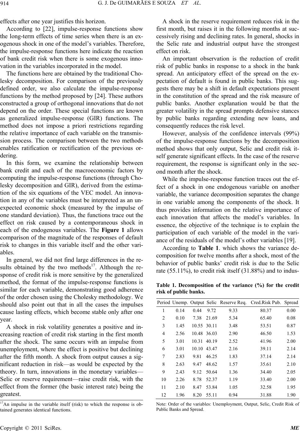

G. J. De GUIMARÃES E SOUZA ET AL.
914
effects after one year justifies this horizon.
According to [22], impulse-response functions show
the long-term effects of time series when there is an ex-
ogenous shock in one of the model’s variables. Therefore,
the impulse-response functions here indicate the reaction
of bank credit risk when there is some exogenous inno-
vation in the variables incorporated in the model.
The functions here are obtained by th e traditio n al Cho-
lesky decomposition. For comparison of the previously
defined order, we also calculate the impulse-response
functions by the method proposed by [24]. These authors
constructed a group of orthogonal innovations that do not
depend on the order. These special functions are known
as generalized impulse-response (GIR) functions. The
method does not impose a priori restrictions regarding
the relative importance of each variable on the transmis-
sion process. The comparison between the two methods
enables ratification or rectification of the previous or-
dering.
In this form, we examine the relationship between
bank credit and each of the macroeconomic factors by
computing the impulse-response functions (through Cho-
lesky decomposition and GIR), derived from the estima-
tion of the six equations of the VEC model. An innova-
tion in any of the variables must be interpreted as an un-
expected economic shock (measured by the impulse of
one standard deviation). Thus, the functions trace out the
effect on risk caused by a contemporaneous shock in
each of the endogenous variables. The Figure 1 allows
comparison of the magnitude of the responses of default
risk to changes in this variable itself and the other vari-
ables.
In general, we did not find large differences in the re-
sults obtained by the two methods17. Although the re-
sponse of credit risk is more sensitive b y the generalized
method, the format of the impulse-response functions is
similar for each variable, demonstrating good adherence
of the order chosen using the Cholesky methodology. We
should also point out that in all the cases the impulses
cause lasting effects, which become stable only after one
year.
A shock in risk volatility generates a positive and in-
creasing reaction of credit risk starting in the first month
after the shock. The same occurs with an impulse from
unemployment, where the effect is po sitive but declining
after the fifth month. A shock from output causes a sig-
nificant reduction in risk—as would be expected by the
theory. In turn, innovations in the monetary variables—
Selic or reserve requirement—raise credit risk, with the
effect from the former (the basic interest rate) being the
greatest.
A shock in the reserve requirement reduces risk in the
first month, but raises it in the following months at suc-
cessively rising and declining rates. In general, shocks in
the Selic rate and industrial output have the strongest
effect on risk.
An important observation is the reduction of credit
risk of public banks in response to a shock in the bank
spread. An anticipatory effect of the spread on the ex-
pectation of default is found in public banks. This sug-
gests there may be a shift in default expectations present
in the constitution of the spread and the risk measure of
public banks. Another explanation would be that the
greater volatility in the spread prompts defensive stances
by public banks regarding extending new loans, and
consequently reduces th e risk level.
However, analysis of the confidence intervals (99%)
of the impulse-response functions by the decomposition
method shows that only output, Selic and credit risk it-
self generate significant effects. In the case of the reserve
requirement, the response is significant only in the sec-
ond month after the shock.
While the impulse-response func tion traces out the ef-
fect of a shock in one endogenous variable on another
variable, the variance decomposition separates the change
in one variable among the components of the shock. It
thus provides information on the relative importance of
each innovation that affects the model’s variables. In
essence, the objective of the technique is to explain the
participation of each variable of the model in the vari-
ance of the residual s of the model ’s ot h er variable s [19].
According to Table 1. which shows the variance de-
composition for twelve months after a shock, most of the
behavior of public banks’ credit risk is due to the Selic
rate (55.11%), to credit risk itself (31.88%) and to indus-
Table 1. Decomposition of the variance (%) for the credit
risk of public banks.
PeriodUnemp.OutputSelicReserve Req. Cred.Risk Pub.Spre a d
1 0.140.449.729.33 80.37 0.00
2 0.107.3821.695.34 65.40 0.08
3 1.4510.5530.113.48 53.51 0.87
4 2.5610.4836.032.90 46.50 1.53
5 3.0110.3140.192.52 41.96 2.00
6 3.0110.1043.472.16 39.11 2.14
7 2.839.8146.251.83 37.14 2.14
8 2.639.4748.621.57 35.61 2.10
9 2.439.1250.641.36 34.40 2.05
10 2.268.7852.371.19 33.40 2.00
11 2.108.4753.841.05 32.58 1.95
12 1.968.2055.110.94 31.88 1.90
17An impulse in the variable itself (risk) to which the response is ob-
tained generates identical functions. Note: Order of the variables: Unemployment, Output, Selic, Credit Risk of
ublic Banks and Spread. P

G. J. De GUIMARÃES E SOUZA ET AL.
915
Figure 1. Response of risk to impulses (one SD) in the other variables—public banks.
trial output (8.20%). The other variables have similar
lesser effects: unemployment (1.96%), spread (1.90%)
and reserve requirement (0.94%). So, the results found
from the impulse-response function and variance de-
composition show that the main macroeconomic deter-
minants of credit risk for public banks in Brazil are the
Selic rate and output. While a positive shock in the for-
mer raises the credit risk, such a shock in the latter low-
ers the credit risk.
3.2. VEC Model—Private Banks
All the variables involved are I(1), according to Table
A.1. Therefore, the Johansen test can be used to identify
the existence of cointegrating vectors, and if this is con-
firmed, their suggested number. Before doing this, how-
ever, it is necessary to choose the number of lags to be
used. The choice was determined by the set of criteria
presented in Table A.4.
Although there was no unanimity among the lag selec-
tion criteria, the choice was the lowest (two lags in the
vector autoregression model and one by the cointegration
test), since this was indicated by the majority of the cri-
teria to determine the lags (AIC, SC and HQ), by the
methodology of [18], by the SC and AIC criteria of the
underlying model and by the parsimony principle to-
gether with analysis of the residuals.
The option to use the constant and trend in the cointe-
grating relation and the constant in the VAR is based on
the Schwarz and Akaike criteria from graphical analysis
of the variables involved. The specification of the deter-
ministic components utilized in the cointegration con-
verges with that employed in the error correction model
for private banks. This definition suggests, at 5% statis-
tical significance, the existence of a cointegration vector
according to the tests of the trace and maximum eigen-
value. Faced with this, we decided to analyze the dy-
namic interactions of these variables in the context of a
VEC model.
We examine the robustness of the model by means of
a set of tests. Regarding autocorrelation, the Portmanteau
and Lagrange multiplier tests do not present significant
indications (at 99% confiden ce) of existen ce. Visual ana-
lysis of the residuals corroborates this evidence. By the
White tests, with and without addition of crossed terms,
there are no reasons to reject the hypothesis of homo-
scedastic residuals. At a 1% significance level, the nor-
mality of the residuals is rejected by the Lutkepohl test,
but not rejected by the Doornik-Hansen test. The six en-
dogenous variables and the cointegrating vector impose
five eigenvalues on the unit circle. However, the other
eigenvalues have absolute values less than one. There-
fore, the results validate the specificatio n of the proposed
model, allowing proceeding with the specific analyses of
the impulse-response functions and variance decomposi-
tion.
To define a statistically consistent order, we employ
the Granger causality/block exogeneity Wald tests, which
are useful to determine the order of the variables accord-
ing to the degree of exogeneity (Table A.5).
According to the table, the order for private banks is
the following: reserve requirement, unemployment, Selic
rate, industrial output, spread and credit risk. The vari-
able of interest—credit risk—is consequently the most
endogenous. In line with the structure of Equation (2),
the credit risk of private banks is influenced by all the
other series (including the spread), responding to shocks
in the same period. Besides this, the order suggested,
although not determined a priori by the theory, is coher-
ent with it. The level of the reserve requirement is the

G. J. De GUIMARÃES E SOUZA ET AL.
916
most exogenous variable, since it is partly controlled by
the BCB; the bank spread is affected by the macroeco-
nomic factors selected, as is suggested by various studies
of the Brazilian market; industrial output is affected by
monetary policy and unemployment; and private banks’
credit risk is influenced by the economic conjuncture.
For the same reasons presented for the impulse and
variance analyses of public banks, we use a twelve-
month horizon for priv ate institutions. Below the simula-
tions are presented of shocks from the variables involved
in the model private banks’ credit risk. The aim is to
identify the behavior of the credit risk in the face of im-
pulses and at the same time the persistence of these ef-
fects. The responses of private banks’ credit risk to
shocks from each variable in the model are shown in
Figure 2.
The order used for the Cholesky decomposition gener-
ates similar functions to the general impulse-response
(GIR) functions18, which in turn minimizes the possible
composition effects present in the orthogonal shocks. In
general, the responses stabilize seven months after the
simulated innovation.
The credit risk reacts positively after the shock in its
volatility, but this effect declines with time, returning to
a stationary stage. A simulated impulse from unemploy-
ment causes the risk to rise in the first three months, but
this effect reverses in the months thereafter. Nevertheless,
this effect is very near zero.
An output shock reduces the risk significantly both in
the short and long range. The shocks produced by any of
the monetary variables cause permanent elevations in
private banks’ credit risk, but in terms of magnitude, the
effects generated by the Selic rate and reserve require-
ment are stronger than those of the spread. The same
intensity is observed, in the opposite direction, from an
output shock. In the case of private banks, the results
corroborate those that wou ld be expected theoretically.
The macroeconomic factors that cause significant re-
sponses (99% confidence) are output, the Selic rate and
the reserve requirement.
The second step of the examination of private banks
by multiple equations concentrates on decomposition
analysis of the variance of the prediction errors. This is
useful by showing the evolution of the dynamic behavior
of the variables over n periods in the future.
The variance decomposition analysis (Table 2) indi-
cates that the most important variables to explain the
variance in bank credit risk twelve months after a shock
are, besides the risk itself (36.97%), the reserve require-
ment (26.65%), output (18.26%) and the Selic rate
(13.05%). The percentage referring to the spread remains
at roughly four over a period of one year. The part of the
variance explained by unemployment begins to fall after
the second month, reaching 0.68% twelve months after a
shock.
From joint examination of the responses to impulses
and variance decomposition, it can be concluded that the
most important macroeconomic variables in determining
private banks’ credit risk in Brazil are the reserve re-
quirement, Selic rate and industrial output.
3.3. VEC Model—A Bank Comparison
The analyses carried out by the VAR model with error
correction show that output and the Selic rate are deter-
mining factors of bank credit risk in Brazil, irrespective
of the type of bank (public or private). Monetary tight-
ening, measured by a rise in the reserve requirement,
positively affects the risk level of all the cou ntry’s banks,
but the effect is stronger on private banks. Figure 3 and
Figure 4 visually summarize the results obtained by the
general impulse-response (GIR) function and the vari-
ance decomposition analyses for public and private
banks, respectively.
As can be seen from the GIR functions shown in Fig-
ure 3, among the macroeconomic factors the strongest
impacts on public banks’ credit risk (positive and nega-
tive, respectively) are caused by shocks in the Selic rate
and output. They also stand out in explaining the vari-
ance, besides the effect of the risk itself.
For private banks (Figure 4), the macroeconomic fac-
tors that stand out are the reserve requirement, output
and the spread. The spread, despite having the weakest
effect of the three, is positively related to risk, as would
be expected, due to the anticipatory factor. Unemploy-
Table 2. Decomposition of the variance (%) for the credit
risk of public banks.
PeriodReserve Req.Unemp.Selic Output Spread Cred. Risk Priv.
1 0.08 0.752.04 0.02 1.25 95.86
2 0.98 3.721.07 3.06 1.32 89.85
3 6.27 2.770.65 13.79 2.30 74.22
4 12.55 1.900.69 19.45 4.20 61.22
5 16.85 1.521.53 21.46 5.17 53.47
6 19.68 1.303.06 21.57 5.38 49.00
7 21.59 1.144.91 21.09 5.25 46.02
8 23.02 1.006.78 20.47 5.05 43.68
9 24.18 0.898.56 19.86 4.85 41.67
10 25.15 0.8010.19 19.29 4.68 39.89
11 25.96 0.7311.69 18.76 4.53 38.33
12 26.65 0.6813.05 18.26 4.39 36.97
18In the case of a shock in the risk itself, the functions overlap in Fig-
ure 2. Note: Order of the variables: Reserve Requirement, Unemployment, Selic,
utput, Spread and Credit Risk of Private Banks. O

G. J. De GUIMARÃES E SOUZA ET AL.
917
Figure 2. Response of risk to impulses (one SD) in the other variables – private banks.
Figure 3. Impact and variance—credit risk of public banks.
Figure 4. Impact and variance—credit risk of private banks.
ment showed a weak cyclical effect on private banks’
credit risk. Therefore, the results of the impulse-response func- tions and variance decomposition suggest that the basic

G. J. De GUIMARÃES E SOUZA ET AL.
918
interest rate and level of economic activity are the main
macroeconomic determinants of bank credit risk in Bra-
zil. If on the real side the effects on credit risk of changes
in output stand out in relation to unemployment, on the
monetary side the Selic rate prevails over the other vari-
ables due to its strong link with the other macroecono mic
factors. Besides, since June 1999 the inflation targeting
regime was adopted in Brazil, and the main instru ment to
the disposition of the BCB for the convergence of infla-
tion to the target is the Selic. Reference [25] suggests
that the process of building credibility in Brazil is slow,
and therefore, a lower credibility implies higher varia-
tions in the interest rate for controlling inflation in Bra-
zil.
It can also be seen that public b anks are more sensitiv e
to macroeconomic fluctuations than are private banks.
The impact of factors of the structural scenario is stronger
on public banks.
The next section examines the process of interaction
between banks and the macroeconomic dynamic. This
interactivity can be one of the causes of the distinct ef-
fect on credit risk between the two types of banks.
4. Macro and Micro Risk—Analysis by
Cointegration
Structural factors affect the risk banks run on their loan
portfolios. However, this risk is not only imposed by the
economic scenario, but also by the intrinsic characteris-
tics of their borrowers and the banks themselves. This
combination of microeconomic factors is called idiosyn-
cratic risk.
Financial institutions, in the face of the level of eco-
nomic uncertainty, change their stance regarding selec-
tion of borrowers and supply of loans to presage possible
changes in the level of default. This is the gist of the
question. Banks are totally pro-cyclical, meaning they
are more selective in their lending during periods of
greater economic uncertain ty, and vice versa. The partial
control over the profile of their loan portfolios enables
banks to maintain the risk level within an interval pre-
established by them. This control occurs through the
idiosyncratic risk of the loan portfolio—through the ca-
pacity to choose borrowers according to their risk profile—
allowing banks to offset the effects of the macroeconomic
environment19. Economic downturns prompt banks to
take a defensive stance in offering credit and raise the
bar for borrowers. The opposite happens in times of
strong growth and reduced macroeconomic uncertainties:
banks increase their lending and lower the bar for bor-
rowers20.
From a standpoint of managing assets according to li-
quidity, it can be argued that banks, in accompanying the
economic cycle, direct their investments considering not
only yield, but also maturity profile, liquidity and uncer-
tain. In economic slowdowns, banks reduce their lending
and/or shift their resources to other types of assets, rais-
ing their average position in more liquid assets and re-
ducing their leverage. In periods of strong growth they
prefer yield over liquidity. In other words, banks can be
expected to increase their risk exposure in growth phases,
becoming more willing to accept lower risk exposure
margins of firms, while in crisis moments they tend to
increase their preference for liquidity, independent of the
expected returns from their investment projects.
Then, infers that banks have a relevant role in ex-
plaining the behavior of the economic cycle, both by
accommodating demand for credit in upturns, spurring
economic activity, and by contracting credit during
downturns, worsening the crisis by restricting lending to
companies because of their deteriorated capacity to gen-
erate cash flow.
Therefore, credit risk, besides its structural component
dictated by the macroeconomic environment, is associ-
ated with the idiosyncratic aspects of borrowers them-
selves. Banks, although they have influence, do not have
control over macroeconomic variables. However, they
can change the profile of their loan portfolios to lower
their risks.
Consequently, banks – although they are affected by
macroeconomic risk – only can directly interfere in the
microeconomic risk of their loan portfolios. This partial
control over idiosyncratic risk, in the ambit of the po rtfo-
lio, can be used to offset changes in the situational risk21.
Increases in macroeconomic risk induce counterpart ac-
tions by banks to lower their microeconomic risk and
thus to maintain their overall risk at the desired levels
established by management. Banks thus act to efficiently
manage the risk/return ratio of their lending operations.
We also investigate this phenomenon in Brazil in the
study period. The credit risk measured in this paper, ac-
cording to the methodology followed, refers to the total
credit risk, i.e., both the macro and microeconomic risk.
It is the risk of loan default of the portfolio, considering
the characteristics of borrowers and the economic envi-
ronment in which they are inserted22.
19Control over the profile of the loan portfolio is heightened in situa-
tions where the supply of credit is lower than demand and competition
is imperfect, as occurs in Brazil.
20The credit cycle follows the economic cycle. This association, in-
cluding for Lat i n America, is discussed i n [ 2 6 ].
21Although it is impossible for banks to alter the idiosyncratic risk o
f
each borrower/loan, they can modify the idiosyncratic risk at the port-
folio level, i.e., the microeconomic risk involved in the total loan port-
folio.
Despite the theoretical knowledge of the separation of
22Banks’ internal models to determine the probability of default must
take these factors into consideration according to the applicable regula-
tions.

919 G. J. De GUIMARÃES E SOUZA ET AL.
risk into macro and micro components, their analytic
division is complicated. Formulation of a standard meas-
ure of idiosyncratic risk of the loan portfolio separate
from macroeconomic risk is not simple, despite the sta-
tistical and mathematical advances regarding risk. Here
we employ measures that demonstrate the loan portfolio
movements induced by banks aiming to modify their
total idiosyncratic risk.
However, there is also the difficulty of obtaining in-
formation on loan portfolios broken down by type of
control in Brazil. The most detailed data refer to credit
operations with non-earmarked funds. However, at this
level of information there is no segmentation by type of
bank. For this reason, we first decided to analyze the
cointegration relation between the micro and macro risk
for the entire sample of banks, and then with another set
of proxies to analyze this by type of bank. If it is not
possible to capture the idiosyncratic risk directly, various
indicators that measure banks’ posture regarding changes
in idiosyncratic risk can be employed as proxies.
We measure the oscillations in microeconomic risk for
banks in Brazil by two loan origination series: LLEND-
TOASSETS_SA and LPERLOANIND_SA. We also
separately use proxies to capture the movements in the
loan portfolios of public and private banks to change
their microeconomic risk: the amount of real lending
transactions (LREALCREDPUB_SA and LREA CRED-
PRIV_SA) and the percentage of the portfolio dedicated
to loans to individuals (LPERCINDPUB_SA and LPER-
CINDPRIV_SA).
In light of the empirical literature [27], we use the
country risk (LEMBI) as a proxy for macroeconomic risk.
We contrast this risk series with each of the proxies for
changes in the idiosyncratic risk.
It is known that changes in a bank’s lo an portfolio are
slow, given the intrinsic characteristics of loans. There is
a delay between the repayment of existing loans and ex-
tension of new ones according to the latest policies de-
fined by management. Therefore, changes in loan portfo-
lio makeup in principle only occur over the medium and
long term. To verify the relationship of two variables
over the long run, cointegration analysis can be used .
We check the cointegration of the series according to
the model of [16,17], which uses a VAR. We know in
advance that the series involved are first-order integrated
processes, so cointegration can be applied. If the series
are cointegrated, a long-run relationship can be said to
exist between them, and the cointegration vector coeffi-
cients are long-term elasticities of banks’ reaction to
changes in the macroeconomic risk.
4.1. Macro and Micro Risk Relation—All Banks
We verified the cointegration between macroeconomic
risk and lending levels in relation to bank assets and be-
tween macro risk and the percentage of loans to indi-
viduals for all banking institutions in the country.
4.1.1. Relation between Country Risk and Loans to
Assets Ratio
A bank, just as any other agent whose activity is specula-
tive and demands some degree of protection, composes
its portfolio seeking to conciliate profitability with its
preference for liquidity, which entails its precaution re-
garding the uncertainty of the results. Therefore, the
composition of a bank’s assets depends on its willingness
to absorb risks associated with uncertain future events,
more specifically the state of its expectations about these
events. When the bank’s evaluation is unfavorable about
the future return on loans, maintenance of the value of
the collateral required and behavior of market interest
rates, it will likely prefer more liquid assets to traditional
loans, which normally have a longer maturity profile.
These decisions are related to the administration of the
bank’s bala nc e sheet.
The series on credit transactions covers loans con-
tracted at interest rates freely set by banks according to
what borrowers are willing to pay23. It does not include
farm credit transactions, onlending from the National
Bank for Social and Economic Development (BNDES)
or any other loans from government sources or compul-
sory reserve deposits. This series weighted by the series
on bank asset levels thus gives the percentage of loans in
relation to assets. An increase in lending only because of
higher assets and a decrease because of lower assets is
controlled. Therefore, in response to oscillations in the
macroeconomic scenario, banks can extend more or less
credit, and part of banking funds can be invested in other
assets with differentiated risk profile instead of to make
traditional loans.
The proxies used in this subsection for the micro and
macroeconomic risks are, respectively, LLENDTOAS-
SETS_SA and LEMBI. These series have a linear corre-
lation of negative 0.39. To estimate the cointegration
vectors by the Johansen approach, we use a VAR model,
with the number of lags chosen according to the majority
of the criteria: LR, FPE, AIC, SC and HQ (Table A.6).
These choices are in line with the parsimony principle.
The possible inclusion of deterministic terms in the
VAR and the cointegration equation is d etermined by the
Schwarz and Akaike criteria and by graphical analysis of
the variables. In the case here, we chose not to assume a
23The series on lending and volume by type of borrower refer to r ef er to
transactions in the National Financial System. However, the high rep-
resentation in this system (99.07% of total assets, with the fifty largest
banks responsible for 83.90%), ensures the quality of the proxy. The
data are from June 2006 (available at the BCB site).

G. J. De GUIMARÃES E SOUZA ET AL.
920
linear trend in the data and to include the constant on ly in
the cointegration relation. This configuration indicates
(at 5% statistical significance) the existence of a cointe-
gration relationship both by the trace statistic and the
maximum eigenvalue (Table A.7).
After choosing the most suitable specification for the
VAR by the criteria adopted and its subsequent approval
by the robustness tests, we applied the Johansen model to
estimate the cointegrating vector. The long-term relation
between the ratio between lending and assets and macro
risk can be described as shown bel o w24:
(0.14) (0.01)
LLENDTOASSETS_SA2.97 0.04LEMBI (4)
The sign for the macroeconomic risk is negative,
which is the first indication of the assumed hypothesis.
4.1.2. Relation between Country Risk and Loans to
Individuals
According to [28] page 135, [...] a bank’s decision prob-
lem is how to distribute the resources they create or col-
lect among these different items that offer specific com-
binations of expected monetary returns and liquidity
premia, instead of just choosing between reserves and
loans or of passively supplying whatever amount of
credit is demanded.
The idea of managing assets according to illiquidity
risk present in [29] can be extrapolated to credit risk.
Given that the total amount of credit offered is mainly
defined by the amount of reserves, choosing the constitu-
tion of the loan portfolio according to the different types
of borrowers and their respective idiosyncratic risks is
essential in managing the risk of banking assets, i.e., the
overarching decision is not how much to lend, but to
which borrowers.
Therefore, banks can make changes in their micro-
economic risk by varying the profile of their loans. Ce-
teris paribus, changes in the loan portfolio composition
can cause reductions or increases in microeconomic risk,
and hence changes in overall risk.
It is known a priori that the default risk on loans to in-
dividuals is substantially higher than on loans to compa-
nies. Therefore, alterations in the portfolio percen tage by
type of borrower change the portfolio’s idiosyn cratic risk
profile. It is reasonable to expect that rises in the macro-
economic risk induce reduction in the microeconomic
risk, through a reduced percentage of personal loans in
relation to business loans, and vice versa25.
The two proxies used here are LPERLOANIND_SA
for micro risk and LEMBI for macro risk. There is a
strong negative linear correlation between them (–0.79).
We use a VAR model to verify the existence of cointe-
gration and estimate the possible vector(s). The joint
analysis of the LR, FPE, AIC, SC and HQ criteria,
shown in Table A.8, indicates the use to two lags. From
visual analysis of the series, which suggests there is no
deterministic trend in the data, along with application of
the Schwarz criterion, we include the constant in the
cointegration relation. Regarding the number of cointe-
gration vectors, both the trace and maximum eigenvalue
statistics indicate (at 5% significance) one vector (Table
A.9).
The normalized coefficients of the cointegration rela-
tion are shown in Equation (5) and represent the long-
term relationship.
(0.06) (0.00)
LPERLOANIND_SA0.80 0.05LEMBI (5)
The contrary reaction through alterations in the loan
portfolio composition is confirmed by the significance of
the estimated coefficient. The value of this coefficient is
similar to that found in estimation via th e prox y LLEND-
TOASSETS_SA.
4.2. Macro and Micro Risk Relation—By Type
of Bank
As can be observed, the structural factors influence the
risk profile of banks’ loan portfolios. This influence has
some specificities regarding type of ownership. Private
Banks are affected differently than ones controlled by the
government.
On the matter of partial control of idiosyncratic risk,
private banks have more flexibility than public ones in
adjusting the risk composition of their portfolios. The
greater freedom to choose assets and borrowers with the
sole purpose of maximizing profits favors the risk/return
strategies of private banks. Therefore, we also analyze
the level of risk according to type of finan c ial institution.
However, it is not possible to use the same series as
before to capture changes in microeconomic risk, be-
cause the series are not available broken down to this
level. To overcome this limitation, we use series on
lending transactions in general and lending to individuals,
both of which are available by type of bank.
4.2.1. Relation between Country Risk and Lending
Transactions by Type of Bank
Although we are not working with n ew loan or ig inations,
a bank’s total amount of credit is to a large measure de-
fined by these. The total amount of loans is managed by
the bank to ensure the expected return given the risk and
to protect itself against changes in the macroeconomic
24The (normalized) coefficients and standard deviation are in parenthe-
ses.
25The change in the micro-risk also occurs due to the change in concen-
tration by ty p e o f b o rrower.

921 G. J. De GUIMARÃES E SOUZA ET AL.
scenario. The series employed (LREALCREDPUB_SA
and LREALCREDPRIV_SA) reflect the total amount
banks (public and private, respectively) choose to keep
under their tutelage. Therefore, the economic scenario
determines the overall credit limit of the banking institu-
tion, or its maximum risk e xpo sure.
The new loans made in the final analysis depend on
the volume of credit already made available. This credit
series reflects the flow of credit transactions. It can thus
be considered as a net series, i.e., the new loans made in
the period minus amortizations of existing loans. There-
fore, changing the (real) volume of credit at risk is an-
other way banks react to the effects from the macroeco-
nomic scenario.
4.2.1.1. Relation of Credit Transactions for Public Banks
The series used are LREALCREDPUB_SA for micro
risk and LEMBI for macro risk. The correlation is nega-
tive 0.20, meaning there is no strong evidence of time
precedence. The order of the VAR is defined according
to Table A.10.
The choice to include the intercept only in the cointe-
gration relation is due to the Schwarz criterion and to th e
behavior of the series in question. The trace statistic and
maximum eigenvalue do not indicate the presence of
cointegration (Table A.11)26. Consequently, according to
the Johansen procedure, no long-term relationship can be
found for the public ba nking sector.
4.2.1.2. Relation of Credit Transactions for Private
Banks
The difference in relation to the preceding sub-item is the
seasonally adjusted logged series of real lending transac-
tions of private banks, or LREALCREDPRIV_SA. The
linear correlation between this and the micro risk meas-
ured by LEMBI is negative 0.29. Table A.12 presents
the statistics that permit determining the number of lags
in the VAR. We chose the suggestion of the SC and HQ
and thus lost fewer degrees of freedom.
The results of the tests suggest that the best model
should include a constant in the cointegration relation
and the VAR and a trend only in the cointegration vector.
We ran various tests to ensure the robustness of the
model. With this specification, both the trace and maxi-
mum eigenvalue tests (Table A. 13) indicate the presence
of cointegration. Based on this, the normalized coeffi-
cients for the cointegration relation can be calculated by
the Johansen procedure. The equation can be expressed
as follows:
(0.58)(0.01)
LREALCREDPRIV_SA3.06LEMBI 0.04TREND


(6)
Therefore, the analysis of private banks corroborates
the long-term relationship between micro and macro risk.
4.2.2. Relation between Country Risk and Percentage
of Loans to Individuals by Type of Bank
In periods of economic euphoria, banks tend to look for
yield over safety, subjecting their assets to greater per-
ceived risks but higher returns. In economic slumps, the
opposite happens: banks direct their assets to less profit-
able but also less risky op erations.
An increase in the concentration of loans to individu-
als, a priori, causes higher (idiosyncratic) risk of default,
mainly due to th e profile of these borrower s, who have a
greater tendency for nonpayment27. According to this
pattern, banks should reduce their exposure to personal
loans when the structural risk increases.
4.2.2.1. Percentage of Loans to Individuals by Public
Banks
The correlation between the percentage of loans to indi-
viduals (LPERCINDPUB_SA) by public banks and
macroeconomic risk is negative 0.30. The statistics (Ta-
ble A.14) determine the number of lags used in the VAR
model. Both information criteria used (AIC and SC) in-
dicate only the inclu sion of the constant in th e cointegra-
tion relation, a choice that is validated by visual analysis
of the series.
Both the test statistics (trace and maximum eigenvalue)
showed in Table A.15 reaffirms the inexistence of a
cointegrating relation for public banks.
4.2.2.2. Percentage of Loans to Individuals by Private
Banks
For private banks the negative correlation between mac-
roeconomic risk and the percentage of loans to individu-
als is high (–0.74). The joint analysis of the LR, FPE,
AIC, SC and HQ criteria unanimously indicates the
number of lags (Table A.16), while in the choice of the
deterministic terms, the AIC and SC present conflicting
results. The SC indicates only inclusion of the constant
in the cointegration relation, while the AIC proposes
including an intercept as well in the VAR. However,
visual inspection of the series suggests the presence of a
linear trend, and hence we chose to follow the Akaike
criterion.
26The idea is ratified by the absence of cointegration by any of the
p
ossible configurati o n s.
27If on the one hand the funds are dispersed in a greater number o
f
borrowers, on the other there are negative effects of concentration in
one type of portfolio, less collateral per customer/transaction and high-
er operating cost per loan, for example.
The trace and maximum eigenvalue tests evidence the
presence of cointegration between the two risk levels

G. J. De GUIMARÃES E SOUZA ET AL.
922
incurred on lending operations, but also banks’ reactions
ed that macroeconomic factors signifi-
ca
the only effects. Banks are
ec
scenario affect the av-
er
also found evidence of differences in this interac-
tiv
extent the characteristics that distinguish
ea
(Table A.17)28. Therefore, the Johansen method allows
estimating the coefficients of the long-term relation.
(0.04)
LPERCINDPRIV_SA 0.32LEMBI (7)
Once again, the relation is significant and negative for
private banks, unlike the pattern for public institutions.
Additionally, the results of the negative long-term rela-
tion are stronger—in terms of the value of the estimated
coefficient—for the sub-sample of private banks than for
all banks. Hence, this shows that the relation observed
for banks in general is to a great extent influenced by the
behavior of private banks.
This different reaction by government-controlled banks
in relation to their private peers is coherent with the
characteristics of the two types of banks and with the
results found in the VEC models. The more rigid defini-
tion of the volume of credit by public banks makes them
more susceptible to changes in the macroeconomic situa-
tion. As observed in the previous sections, the impact on
credit risk from macroeconomic factor s is more sensitive
in the portfolios of public banks. Th e lesser flexibility of
public banks to define the volume of credit and deter-
mine the profile of the portfolio restricts their ability to
adjust to the macroeconomic environment.
In overall terms, both from the standpoint of origina-
tion of loans—used for banks in general—and from the
standpoint of exposure to credit risk—broken down by
bank type—we found there is an interaction between the
economic situation and banks in constitution of credit
risk at the portfolio level. This is what composes the
spread and determines the average in terest rate on loans.
5. Conclusions
According to the [7] page 45, in th e case of Brazil, wh e r e
the capital and private bond markets are relatively un-
derdeveloped and restricted to few participants, bank
credit has great relevance in financing companies. The
high cost of this type of credit, therefore, can have nega-
tive implications on the accumulation of capital and
technological innovation, and consequently on economic
growth.
Generally the diagnoses made in the economic litera-
ture point to risk of default as one of the main causes of
the high bank spread in Brazil. In this sense, a better un-
derstanding of bank credit risk can help in management
of economic policy.
This paper investigated the interactive process be-
tween the macroeconomic environment and bank credit
risk, not only in the way structural factors affect the risk
to these effects.
We first observ
ntly impact the credit risk incurred by banks. Despite
the effects caused by unemployment and monetary tigh-
tening, economic growth and the Selic rate stand out as
factors affecting this risk.
However, these are not
onomic agents, and as such they seek to take advan-
tage of the opportunities on offer. To control the idio-
syncratic risk involved in lending operations, these insti-
tutions can—through active measures—modify the size
and/or profile of their loan portfolios. This makes for an
interactive process involving banks, credit risk and the
macroeconomic environment. Figure 5 structurally sum-
marizes the discussion of the relationship between mac-
roeconomic risk and idiosyncratic risk and its impact on
the performance of the economy.
Changes in the macroeconomic
age default risk of loan portfo lios, which in turn modi-
fies the cost structure, spreads and interest rates charged
on loans. As a consequence, the volume of credit changes,
implying variations in economic growth—intrinsically
related to macroeconomic factors. Nevertheless, this cy-
cle depends on the way banks react to economic fluctua-
tions. Modification of the risk of default by determina-
tion of the loan portfolio profile can minimize or even
totally offset the effects from the macroeconomic sce-
nario.
We
e process according to the type of bank control. Banks
in the private sector respond more actively to the impacts
of the macroeconomic situation than do public banks,
enabling them to better mitigate the effects and manage
their loan portfolios more efficiently. Public banks face
greater institutional and legal barriers and often political
pressures as well that hinder a more active risk manage-
ment stance.
To a certain
ch type of bank help explain the differences found in
the relevance and significance of the effects caused by
each macroeconomic factor, the strength and duration of
Figure 5. General summary—the interactive process inr- te
28This cointegration relation is reinforced by the fact it exists regardless
of the specification chosen. fering in the econ omic cy cle.

G. J. De GUIMARÃES E SOUZA ET AL. 923
mic shocks and the reaction
t to shed light on bank
cr
. References
] Banco Central do Brasil, “Juros e Spread Bancário
read 112000. pdf
ancá-
urospread112001.pdf
Bancá-
urospread122002.pdf
Bancá-
econmia_bancaria_credito.
o Central do Brasil, “Relatório de Economia Bancá-
/spread/port/economia_bancaria
do Brasil, “Relatório de Economia Bancá-
d/port/rel_econ_ban_cre
Central do Brasil, “Relatório de Economia Bancá-
/Pec/spread/port/relatorio_economi
ermann, B. J. Treutler and S. M.
Credit Risk
, “X-12-ARIMA: Reference Manual
/srd/www/x12 a
Schmidt and Y.
Edi-
e Series
sis,” 4th Edition, Pren -
Cointegration Vec-
1-3
the impacts caused by econo
itself to structural oscillations with respect to risk. The
reactions measured by exposure to credit risk are sig-
nificant only for private banks. Being controlled by the
government limits the extent of the changes possible in
the loan portfolio composition, and at the same time
makes the average credit risk of public banks more sus-
ceptible to economic variations.
In summary, this paper sough
edit risk in Brazil under new prisms, by examining the
lending risk incurred by banks not only as depending on
the macroeconomic scenario but also the stance of banks
to this risk. This interaction of the macroeconomic envi-
ronment and banks must be considered at the moment of
making economic policy decisions. In terms of regula-
tion, while during crisis moments the defensive posture
of banks can hinder reaching the inflection point of re-
newed growth, in moments of economic expansion the
excessive leverage posture can lead to a crisis in the fi-
nancial sector that spreads to the entire economy it un-
derpins.
6
[1 no t
Brasil,” 1999. http://www.bcb.gov.br/ftp/juros-spread1.pdf
[2] Banco Central do Brasil, “Relatório de Economia Bancá-
ria e Crédito: Avaliação de 1 ano do Projeto Juros e
Spread Bancário,” 2000.
http://www.bcb.gov.br/ftp/jurosp
[3] Banco Central do Brasil, “Relatório de Economia B
ria e Crédito: Avaliação de 2 anos do Projeto Juros e
Spread Bancário,” 2001.
http://www.bcb.gov.br/ftp/j
[4] Banco Central do Brasil, “Relatório de Economia
ria e Crédito: Avaliação de 3 anos do Projeto Juros e
Spread Bancário,” 2002.
http://www.bcb.gov.br/ftp/j
[5] Banco Central do Brasil, “Relatório de Economia
ria e Crédito: Avaliação de 4 anos do Projeto Juros e
Spread Bancário,” 2003.
http://www.bcb.gov.br/ftp/rel_
pdf
[6] Banc
ria e Crédito: Avaliação de 5 anos do Projeto Juros e
Spread Bancário,” 2004.
http://www.bcb.gov.br/Pec
_e_credito.pdf
[7] Banco Central
ria e Crédito. Brasília,” 2005.
http://www.bcb.gov.br/pec/sprea
d.pdf
[8] Banco
ria e Crédito,” 2006.
http://www.bcb.gov.br
a_bancaria_credito.pdf
[9] M. H. Pesaran, T. Schu
Weiner, “Macroeconomic Dynamics and Credit Risk: A
Global Perspective,” Journal of Money, Credit and Ban-
king, Vol. 38, No. 5, 2006, pp. 1211-1261.
[10] A. Cunningham, “Rating Methodology: Bank
in Emerging Markets—An Analytical Framework,” 1999.
http://rating.interfax.ru/data/rating/emerging%20banks%
20methodology.pdf
[11] U. S. Census Bureau
Version 0.3,” 2007.
http://www.census.gov
[12] D. Kwiatkowski, P. C. B. Phillips, P.
Shin, “Testing the Null Hypothesis of Stationary against
the Alternative of a Unit Root: How Sure Are We That
Economic Time Series Have a Unit Root?,” Journal of
Econometrics, Vol. 54, No. 1-3, 1992, pp. 159-178.
[13] G. S. Maddala, “Introduction to Econometrics,” 3rd
tion, John Wiley & Sons Ltd., Chichester, 2001.
[14] H. Lütkepohl, “New Introduction to Multiple Tim
Analysis,” Springer, Berlin, 2005.
[15] W. H. Greene, “Econometric Analy
tice-Hall, Upper Saddle River, 2000.
[16] S. Johansen, “Statistical Analysis of
ors,” Journal of Economic Dynamics and Control, Vol.
12, No. 2-3, 1988, pp. 231-54.
doi:10.1016/ 0165-1889(88)9004
esis Testing of [17] S. Johansen, “Estimation and Hypoth
Cointegrating Vectors in Gaussian Vector Autoregressive
Models,” Econometrica, Vol. 59, No.6, 1991, pp. 1551-
1580. doi:10.2307/2938278
[18] S. G. Hall, “The Effect of Varying Length VAR Models
91.tb00320.x
on the Maximum Likelihood Estimates of Cointegrating
Vectors,” Scottish Journal of Political Economy, Vol. 38,
No. 4, 1991, pp. 317-323.
doi:10.1111/j. 1467-9485.19
Cointegration
/ISSN0195-6574-EJ-Vol21-No1-1
[19] D. F. Hendry and K. Juselius, “Explaining
Analysis: Part I,” Energy Journal, Vol. 21, No.1, 2000,
pp. 1-42.
doi:10.5547
ntegration
SN0195-6574-E J-Vol22-No1 -4
[20] D. F. Hendry and K. Juselius, “Explaining Coi
Analysis: Part II,” Energy Journal, Vol. 22, No. 1, 2001,
pp. 75-120.
doi:10.5547/IS
in Econo-
ers, “Applied Econometric Time Series,” 2nd Edi-
ctions in
Generalized Impulse Re-
[21] R. I. D. Harris, “Using Cointegration Analysis
metric Modelling,” 1st Edition, Prentice-Hall, London,
1995.
[22] W. End
tion, John Wiley & Sons Ltd., New York, 2003.
[23] W. Charemza and D. F. Deadman, “New Dire
Econometric Practice: General to Specific Modelling,
Cointegration and Vector Autoregression,” 2nd Edition,
Edward Elgar, London, 1997.
[24] M. H. Pesaran and Y. Shin, “

G. J. De GUIMARÃES E SOUZA ET AL.
924
sponse Analysis in Linear Multivariate Models,” Eco-
nomics Letters, Vol. 58, No. 1, 1998, pp. 17-29.
doi: 10.1016/S0165-1765(97)00214-0
[25] H. F. de Mendonça and G. J. de Guimarães e Souza, “In-
10
flation Targeting Credibility and Reputation: The Cones-
quences for the Interest Rate,” Economic Modelling, Vol.
26, No. 6, 2009, pp. 1228-1238.
doi:10. 1016/j.econmod.2009.05.0
ries’ Anti-Cy
eference,” In:
ment,
[26] J. A. Ocampo, “Developing Countclical Interest and Money,” Macmillan Press, Cambridge, 1936.
Poli- cies in a Globalized World,” Cepal, Santiago, 2002.
[27] T. S. Afanasieff, P. M. Lhacer and M. I. Nakane, “The
Determinants of Bank Interest Spread in Brazil,” Money
Affairs, Vol. 15, No. 2, 2002, pp. 183-207.
[28] F. J. C. Carvalho, “On Banks’ Liquidity Pr
P. Davidson and J. Kregel., Eds., Full Employment and
Price Stability in a Global Economy, 1st Edition, Edward
Elgar Publishing, Cheltenham, 1999, pp. 123-138.
[29] J. M. Keynes, “The General Theory of Employ

925 G. J. De GUIMARÃES E SOUZA ET AL.
Appendix
Table A.1. Results of the unit root and stationarity tests.
ADF PP DF-GLS KPSS
Series Lag Determ.
comp. Stat Critical
value
10% Lag Determ.
comp. Stat Critical
value
10% Lag Determ.
comp. StatCritical
value
10% Lag Determ.
comp. StatCritical
value
10%
LRISK1PUB_SA 0 C –1.83 –2.59 1 C –1.77–2.590 CT –1.81–2.82 6 C 0.210.35
D(LRISK1PUB_SA) 0 N –9.70 –1.61 0 N –9.70–1.610 CT –9.65–2.82 2 C 0.100.35
LRISK1PRIV_SA 1 C –3.37 –2.59 1 C –2.53–2.591 CT –1.74–2.82 6 C 0.240.35
D(LRISK1PRIV_SA) 0 N –6.65 –1.61 2 N –6.65–1.610 CT –6.44–2.82 1 C 0.250.35
LSELIC 1 C –3.54 –2.59 6 N –0.57–1.61 1 CT –2.60–2.82 6 C 0.130.35
D(LSELIC) 0 N –2.62 –1.61 3 N –2.91–1.61 0 CT –2.64–2.82 6 C 0.080.35
LRESREQ 0 N –1.30
–1.61 3 N –1.26–1.61 0 CT –1.08–2.82 6 CT 0.250.12
D(LRESREQ) 0 N –8.41
–1.61 3 N –8.43–1.61 0 CT –7.61–2.82 3 C 0.210.35
LSPREAD 0 N –0.50
–1.61 2 N –0.50–1.61 0 CT –1.87–2.82 6 C 0.19 0.35
D(LSPREAD) 0 N –9.75
–1.61 1 N –9.74–1.61 1 CT –2.13–2.82 2 C 0.090.35
LEMBI 1 N –0.78
–1.61 4 N –0.73–1.61 1 CT –1.90–2.82 6 CT 0.230.12
D(LEMBI) 0 N –4.94
–1.61 2 N –5.02–2.590 CT –4.69–2.82 4 C 0.210.35
LUNEMP_SA 1 N –0.01
–1.61 3 N –0.02–1.611 CT –1.76–2.82 6 C 0.280.35
D(LUNEMP_SA) 0 N –5.92
–1.61 12N –5.74–1.610 CT –5.89–2.82 3 C 0.160.35
LOUTPUT_SA 3 CT –2.80 –3.61 5 CT –4.64–3.163 CT –2.84–2.82 6 CT 0.180.12
D(LOUTPUT_SA) 1 N –8.98 –1.61 3 N –13.91–1.611
CT –9.21–2.82 4 C 0.050.35
LLENDTOASSETS_SA 2 N 0.43 –1.61 6 CT –6.21–3.162 CT –1.47–2.82 6 CT 0.120.12
D(LLENDTOASSETS_SA) 1 N –11.55–1.61 5 N –20.55–1.611 CT –9.78–2.82 4 C 0.140.35
LPERLOANIND_SA 0 C –2.34 –2.59 3 C –2.12–2.590 CT –3.40–2.82 6 C 0.790.35
D(LPERLOANIND_SA ) 1 N –8.49 –1.61 3 N –10.45–1.611 CT –8.38–2.82 4 C 0.080.35
LREALCREDPUB_SA 2 N 0.65
–1.61 1 N –0.83–1.613 CT –1.57–2.82 6 CT 0.240.12
D(LREALCREDPUB_SA) 1 N –7.68
–1.61 2 N –7.00–1.611 CT –7.99–2.82 1 C 0.220.35
LREALCREDPRIV_SA 3 CT –2.91 –3.16 6 N –4.72–1.61 3 CT –2.10–2.82 6 CT 0.130.12
D(LREALCREDPRIV_SA) 1 C –3.38 –2.59 5 C –7.11–2.591 CT –3.39–2.82 6 C 0.190.35
LPERCINDPUB_SA 0 C –3.05 –2.59 4 C –3.17–2.590 CT –1.18–2.82 6 CT 0.160.12
D(LPERCINDPUB_SA) 0 N –7.66 –1.61 0 N –7.66–1.610 CT –8.11–2.82 1 C 0.410.35
LPERCINDPRIV_SA 0 N –5.07 –1.61 5 N –3.69–1.610 CT –1.22–2.82 6 CT 0.190.12
D(LPERCINDPRIV_SA) 1 C –4.04 –2.59 4 C –7.69–2.591 C –3.06–1.61 5 C 0.120.35
Notes: D( ) is the first difference. The deterministic components are: C = Constant and Linear Trend. In the ADF and DF-GLS tests, the number of lags used
was defined according to the Schwaz criterion. For the PP and KPSS tests we applied selection by Newey-West estimates.
Table A.2. Lag selection criteria—public banks.
Lags LR FPE AIC SC HQ
0 NA 0.00 –17.78 –17.59 –17.70
1 711.24 0.00 –27.72 –26.39 –27.19
2 153.27* 0.00* –29.32* –26.85* –28.33*
3 46.58 0.00 –29.20 –25.59 –27.76
4 43.14 0.00 –29.11 –24.37 –27.23
Notes: The variables used are: Credit Risk (Public Banks), Unemployment, Output, Selic, Reserve Requirement and Spread. The sample corresponds to the
period from March 2000 to June 2006. For the LR, each sequential test uses 5%. (*) Indicates the lag selected by the criterion.

G. J. De GUIMARÃES E SOUZA ET AL.
926
Table A.3. Criterion for ordering the variables—public banks.
Dependent Variable
Unemployment Output Selic Reserve RequirementCredit Ri s k (Public) Spread
Chi-squareProb. Chi-square Prob.Chi-squareProb.Chi-square Prob.Chi-square Prob. Chi-squareProb.
Unemployment - - 1.87 0.170.00 1.001.95 0.161.85 0.17 1.07 0.30
Output 4.68 0.03 - - 0.13 0.720.09 0.763.96 0.05 2.54 0.11
SELIC 0.13 0.72 0.00 0.96- - 0.00 0.987.99 0.00 15.45 0.00
Reserve Requirement 0.72 0.40 1.73 0.193.52 0.06- - 14.69 0.00 14.84 0.00
Credit Risk (Public) 0.37 0.54 3.19 0.070.42 0.520.21 0.65- - 4.73 0.03
Spread 0.15 0.70 2.03 0.152.81 0.094.70 0.039.78 0.00 - -
Total 5.35 0.37 6.64 0.256.77 0.249.87 0.0833.25 0.00 35.95 0.00
Note: Probabili t y values ca l culated by Eviews 5.
Table A.4. Lag selection criteria—private banks.
Lags LR FPE AIC SC HQ
0 NA 0.00 –19.54 –19.35 –19.47
1 692.68 0.00 –29.20 –27.87 –28.67
2 135.01 0.00 –30.54* –28.02* –29.51*
3 55.95* 0.00* –30.49 –26.94 –29.11
4 43.32 0.00 –30.46 –25.72 –28.58
Notes: The variables used are: Credit Risk (Private Banks), Unemployment, Output, Selic, Reserve Requirement and Spread. The sample corresponds to the
period from March 2000 to June 2006. For the LR, each sequential test uses 5%. (*) Indicates the lag selected by the criterion.
Table A.5. Criterion for ordering the variables—private banks.
Dependent Variable
Reserve Requiremen
t
UnemploymentSelic Output Sp read Credit Risk (Private)
Chi-square Prob. Chi-square Prob.Chi-squareProb.Chi-squareProb.Chi-squareProb. Chi-square Prob.
Reserve Requirement- - 3.50 0.065.24 0.021.00 0.327.44 0.01 0.04 0.84
Unemployment 1.92 0.17 - - 0.24 0.632.20 0.142.62 0.11 16.04 0.00
Selic 0.07 0.80 0.23 0.63- - 2.79 0.10 13.59 0.00 9.38 0.00
Output 0.99 0.32 3.95 0.051.06 0.30- - 0.11 0.74 10.21 0.00
Spread 7.19 0.01 0.13 0.721.70 0.195.17 0.02- - 6.58 0.01
Credit Risk (Private) 0.34 0.56 4.61 0.035.81 0.020.00 0.990.13 0.71 - -
Total 12.40 0.03 12.96 0.0213.90 0.0215.73 0.0123.16 0.00 29.59 0.00
Note: The probabilities were calculated by Eviews 5.
Table A.6. Lag selection criteria—loans divided by bank assets.
Lags LR FPE AIC SC HQ
0 NA 0.00 –0.88 –0.81 –0.85
1 198.37 0.00 –3.95 –3.75 –3.87
2 23.88* 0.00 –4.23 –3.90* –4.10*
3 7.32 0.00* –4.23* –3.76 –4.05
4 0.45 0.00 –4.12 –3.52 –3.88
Notes: The variables are: Percentage of Loans Divided by Assets and Country Risk. The sample corresponds to the period from March 2000 to June 2006. For
the LR, each sequential test uses 5%. (*) Indicates the lag selected by the criterion.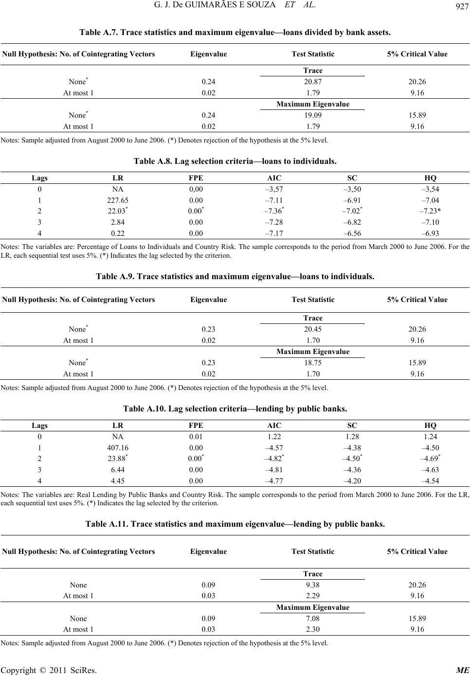

927 G. J. De GUIMARÃES E SOUZA ET AL.
Table A.7. Trace statistics and maximum eigenvalue—loans divided by bank assets.
Null Hypothesis: No. of Co i ntegrating Vectors Eigenvalue Test Statistic 5% Critical Value
Trace
None* 0.24 20.87 20.26
At most 1 0.02 1.79 9.16
Maximum Eigenvalue
None* 0.24 19.09 15.89
At most 1 0.02 1.79 9.16
Notes: Sample adjusted f rom August 2000 to June 2 006. (*) Denotes rejection of the h ypothesi s at the 5% level.
Table A.8. Lag selection criteria—loans to individuals.
Lags LR FPE AIC SC HQ
0 NA 0,00 –3,57 –3,50 –3,54
1 227.65 0.00 –7.11 –6.91 –7.04
2 22.03* 0.00* –7.36* –7.02* –7.23*
3 2.84 0.00 –7.28 –6.82 –7.10
4 0.22 0.00 –7.17 –6.56 –6.93
Notes: The variables are: Percentage of Loans to Individuals and Country Risk. The sample corresponds to the period from March 2000 to June 2006. For the
LR, each sequential test uses 5%. (*) Indicates the lag selected by the criterion.
Table A.9. Trace statistics and maximum eigenvalue—loans to individuals.
Null Hypothesis: No. of Co i ntegrating Vectors Eigenvalue Test Statistic 5% Critical Value
Trace
None* 0.23 20.45 20.26
At most 1 0.02 1.70 9.16
Maximum Eigenvalue
None* 0.23 18.75 15.89
At most 1 0.02 1.70 9.16
Notes: Sample adjusted f rom August 2000 to June 2 006. (*) Denotes rejection of the h ypothesi s at the 5% level.
Table A.10. Lag selection criter i a—le nding by public banks.
Lags LR FPE AIC SC HQ
0 NA 0.01 1.22 1.28 1.24
1 407.16 0.00 –4.57 –4.38 –4.50
2 23.88* 0.00* –4.82* –4.50* –4.69*
3 6.44 0.00 –4.81 –4.36 –4.63
4 4.45 0.00 –4.77 –4.20 –4.54
Notes: The variables are: Real Lending by Public Banks and Country Risk. The sample corresponds to the period from March 2000 to June 2006. For the LR,
each sequential test uses 5%. (*) Indicates the lag selected by the criterion.
Table A.11. Trace statistics and maximum eigenvalue—lending by public banks.
Null Hypothesis: No. of Co i ntegrating Vectors Eigenvalue Test Statistic 5% Critical Value
Trace
None 0.09 9.38 20.26
At most 1 0.03 2.29 9.16
Maximum Eigenvalue
None 0.09 7.08 15.89
At most 1 0.03 2.30 9.16
Notes: Sample adjusted f rom August 2000 to June 2 006. (*) Denotes rejection of the h ypothesi s at the 5% level.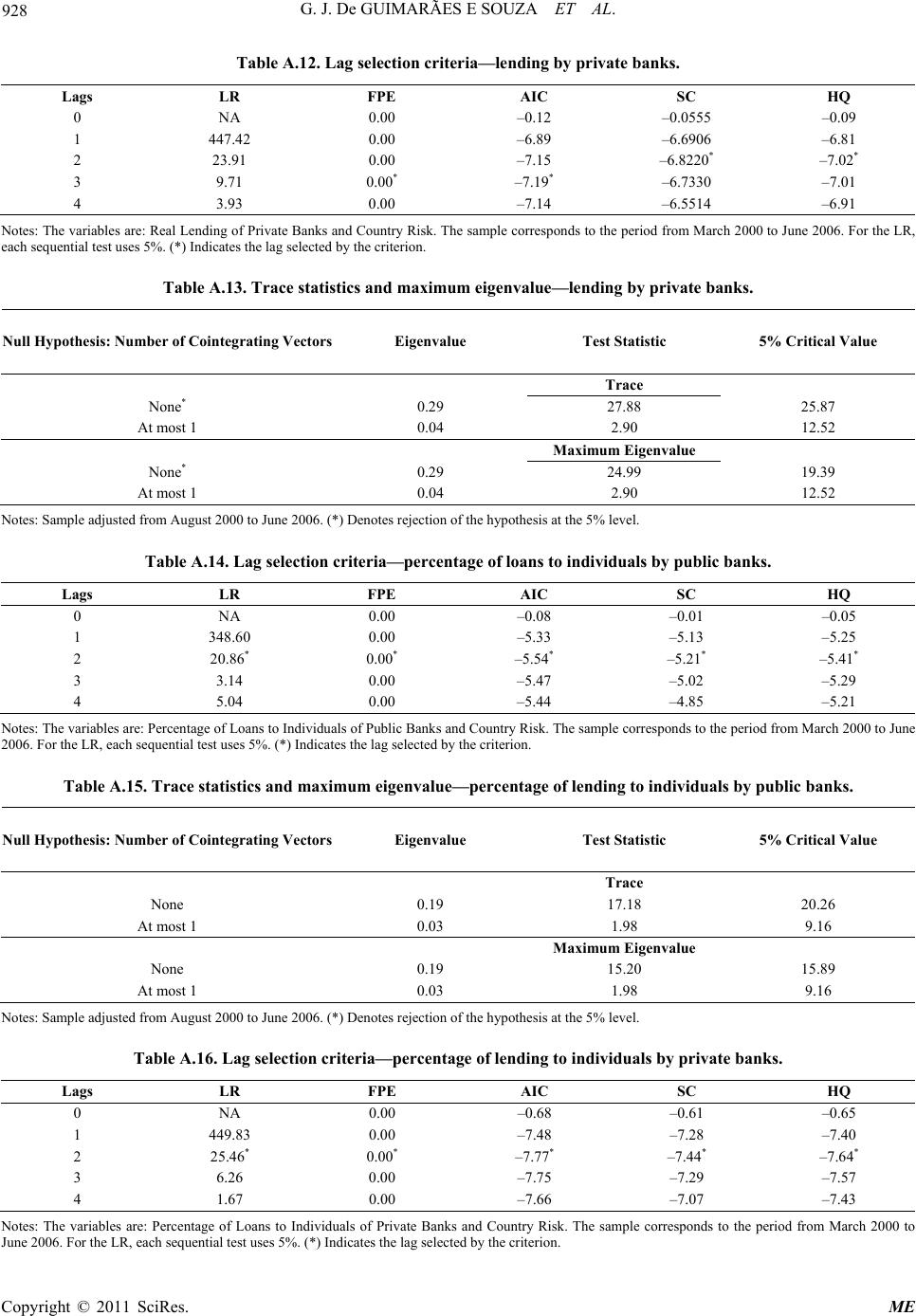

G. J. De GUIMARÃES E SOUZA ET AL.
928
Table A.12. Lag selection criteria—lending by private banks.
Lags LR FPE AIC SC HQ
0 NA 0.00 –0.12 –0.0555 –0.09
1 447.42 0.00 –6.89 –6.6906 –6.81
2 23.91 0.00 –7.15 –6.8220* –7.02*
3 9.71 0.00* –7.19* –6.7330 –7.01
4 3.93 0.00 –7.14 –6.5514 –6.91
Notes: The variables are: Real Lending of Private Banks and Country Risk. The sample corresponds to the period from March 2000 to June 2006. F or the LR,
each sequential test uses 5%. (*) Indicates the lag selected by the criterion.
Table A.13. Trace statistics and maximum eigenvalue—lending by private banks.
Null Hypothesis: Number of Cointegrating Vectors Eigenvalue Test Statistic 5% Critical Value
Trace
None* 0.29 27.88 25.87
At most 1 0.04 2.90 12.52
Maximum Eigenvalue
None* 0.29 24.99 19.39
At most 1 0.04 2.90 12.52
Notes: Sample adjusted f rom August 2000 to June 2 006. (*) Denotes rejection of the h ypothesi s at the 5% level.
Table A.14. Lag selection criteria—percentage of loans to individuals by public banks.
Lags LR FPE AIC SC HQ
0 NA 0.00 –0.08 –0.01 –0.05
1 348.60 0.00 –5.33 –5.13 –5.25
2 20.86* 0.00* –5.54* –5.21* –5.41*
3 3.14 0.00 –5.47 –5.02 –5.29
4 5.04 0.00 –5.44 –4.85 –5.21
Notes: The variables are: Percentage of Loans to Individuals of Public Banks and Country Risk. The sample corresponds to the period from March 2000 to June
2006. For the LR, each sequential test uses 5%. (*) Indicates the lag selected by the criterion.
Table A.15. Trace statistics and maximum eigenvalue—percentage of lending to individuals by public banks.
Null Hypothesis: Number of Cointegrating Vectors Eigenvalue Test Statistic 5% Critical Value
Trace
None 0.19 17.18 20.26
At most 1 0.03 1.98 9.16
Maximum Eigenvalue
None 0.19 15.20 15.89
At most 1 0.03 1.98 9.16
Notes: Sample adjusted f rom August 2000 to June 2 006. (*) Denotes rejection of the h ypothesi s at the 5% level.
Table A.16. Lag selection criteria—percentage of lending to individuals by private banks.
Lags LR FPE AIC SC HQ
0 NA 0.00 –0.68 –0.61 –0.65
1 449.83 0.00 –7.48 –7.28 –7.40
2 25.46* 0.00* –7.77* –7.44* –7.64*
3 6.26 0.00 –7.75 –7.29 –7.57
4 1.67 0.00 –7.66 –7.07 –7.43
Notes: The variables are: Percentage of Loans to Individuals of Private Banks and Country Risk. The sample corresponds to the period from March 2000 to
June 2006. For the LR, each sequential test uses 5%. ( *) Indicate s t he lag selected by the criterion .

G. J. De GUIMARÃES E SOUZA ET AL.
929
Table A.17. Trace statistics and maximum eigenvalue—percentage of lending to individuals by private banks.
Null Hypothesis: Number of Cointegrating Vectors Eigenvalue Test Statistic 5% Critical Value
Trace
None* 0.29 25.91 15.49
At most 1 0.01 0.50 3.84
Maximum Eigenvalue
None* 0.29 25.41 14.26
At most 1 0.01 0.50 3.84
Notes: Sample adjusted f rom August 2000 to June 2 006. (*) Denotes rejection of the h ypothesi s at the 5% level.
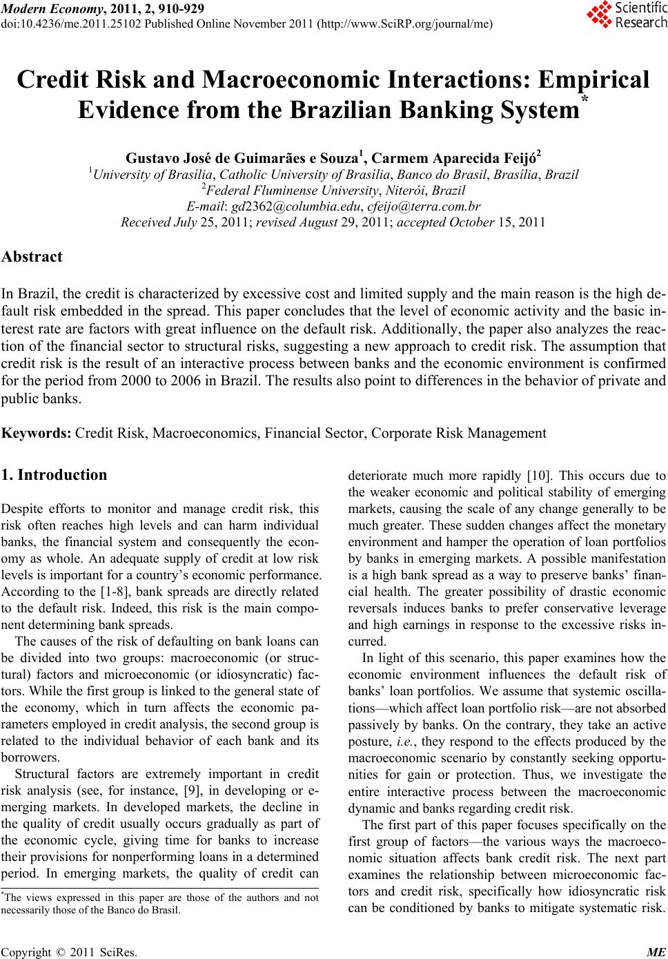