 Modern Economy, 2011, 2, 780-787 doi:10.4236/me.2011.25086 Published Online November 2011 (http://www.SciRP.org/journal/me) Copyright © 2011 SciRes. ME Labor Productivity vs. Minimum Wage Level Mieczysław Dobija Cracow University of Economics, Cracow, Poland E-mail: dobijam@uek.krakow.pl Received August 19, 2011; revised September 17, 2011; accepted October 29, 2011 Abstract Recognition of the abstract nature of capital has liberated some new possibilities for alternative human capi- tal research. Human capital, that is to say the human ability of doing work, is under the authority of all fun- damental laws established in respect of the general notion of capital as spontaneous, and possessing random diffusion and limited growth. The phenomenon of human capital’s natural dispersion is a starting point for the theory of minimum wage, which ought to be sufficient to counterbalance the natural thinning out of the initial human capital of an employee. In practice, the legal minimum wage is fixed at different levels, and sometimes it is very low. Labor productivity is one fundamental factor that enables the establishment of a proper minimum wage level. Each human capital is vanquished by spontaneous and random diffusion, which averages 8% of the initial capital. Therefore the 8% rule is applicable to each employee no matter how edu- cated and experienced he or she is. The results show that the level and fairness of the legal minimum wages is conditioned by labor productivity measured by ratio Q. This ratio should be at least 3.0 so the minimum wage could set off spontaneous random diffusion of employee’s human capital. Keywords: Capital, Human Capital, Minimum Wage, Constant Pay, Labor Productivity 1. Introduction The considerations introduced in this paper belong to an alternative research program of human capital. This re- search differs from T. Shultz’s and G. Becker’s well- known program coined under the popular title, “Invest- ing in People”, as described by M. Blaug [1, pp. 303- 321]. The new program is anchored in a deeper under- standing of capital, which is discerned as the abstract “ability to do work.” The potential growth of capital is determined by the discovered constant p. The kernel of this research program [Lakatos’ hard core] is a model of capital that discloses factors causing changes of the ini- tial capital. In addition to the hard core there is the triad, “capital-labor-money,” where labor is the transfer of capital to objects of work, and money is the pay receiv- ables for work done. Therefore, a labor-driven economy is the central focus of the research program. The model of capital at moment t [2] identifies factors that influence an initial value of capital. Among the fac- tors are ratios s and p, where s measures the spontaneous diffusion of initial capital, and p denotes the economic constant of potential growth. The most important rela- tionship shows that p = Ε(s) = 0.08 [1/year]. Initial capital C0 and time t are the essential factors of the compound interest formula Ct = C0ert. But a true challenge is the theory of the rate (r). As stated by M. Dobija [2] the rate of growth of the initial capital has a three-factor structure. Namely, r = p – s + m, so the ini- tial capital C0 is influenced by the three subsequent fac- tors and flow of time t as follows: ( 00 ee ee) tstmt psmt t CC C and ()0.081/ yearpEs The variables are defined as follows: t—is the coordinating (calendar) time measured by chosen cyclical movements, particularly of the Earth; ept—is the factor of natural potential growth deter- mined by the economic constant p = 0.08; the p also serves as the capitalization rate; e–st—discount factor, s, is the rate of spontaneous and random diffusion of the initial capital; s is a central part of discount rates. emt—is an inflow of capital by human labor and management, which can offset the natural diffusion of capital and can save the potential for growth changing it to profit. Let us note that the variables s and m represent active  781 M. DOBIJA work of the natural forces (–s) and the active outer work that can restrain the dispersion (m). Instead, the constant p symbolizes a potential. The potential p can yield fruit, provided the diffusion s is counterbalanced by the work m. The powerful forces determining our reality become visible in the model of the initial capital changes. Both thermodynamic principles are present here. The first thermodynamic principle is present since the model con- tains initial capital C0. This means that the initial capital can only be changed or transferred but never created. The Second Law is also present since capital constantly diffuses; the initial value spontaneously and randomly declines. The third force that has its part in the game is the natural potential for growth. It is the setup of the Earth and the Sun that guarantees essential potential for growth (p = 8%). Thanks to this potential, human capital grows, originating labor resources. Subsequently, human labor can prevent diffusion by wise, productive labor, setting off dispersion forces and causing that potential growth p to become real economic value1. The model shows, among others, that economy is a non-zero sum game, and the added value can achieve an average rate of 8%. This value concentrates in different resources, both material (goods, soil, devices) and immaterial as intellectual and institutional resources (laws and procedures, among oth- ers). Much research has been done to measure the value of the constant p. This constant manifests in many fields of economic investigation, and is known on the capital mar- ket as the risk premium. A significant research on the subject has been done by B. Kurek [3], who also de- scribed related issues in a recent book “Deterministic Risk Premium Hypothesis” [4, p. 124]. The author found that a good estimator of the constant p is a properly de- fined ROA. Examining financial statements of compa- nies belonging to the S & P 1500 over a 20-year period, the author showed that the average value of ROA = 8%, 28% so the p as a priori value is 8%. Financial state- ments show values at the end of the year so the initial capital compounded at a rate of 0.08 should yield e0.08 = 1.08328, that is to say 8.33%. The author established the confidence interval (8.25; 8.89). Many authors still ex- amine the constant p in the field of employees’ human capital and their compensations. The human capital model and derived compensation models are suitable for testing the fundamental relationship: p = E(s) = 0.08 [1/ year]. For testing, a simple econometric model is suitable. Namely Wa = AWh + B, where Wa is the real pay, and Wh = s × H(T, p) is the pay calculated in line with the human capital model. The variables H(T, p) and T denote re- spectively: H(T, p)—employee’s human capital, and T— years of professional work. Human capital is discerned as an employee’s ability to do work. Models of human capital are derived from the general model, and then compensation models stem from the model of human capital. The most important conclu- sion stemming from the model of capital concerns an amount of fair constant pay. An employee as a living creature has to waste some capital since heat engines working in his body [5, pp. 157-158] have to disperse some energy. To keep balance, the constant pay has to counterbalance this loss. Therefore the constant pay should not be less than 8% of the employee’s human capital (s × H(T, p)). Then the employee’s human capital is maintained, whereas less pay leads to the depreciation of the employee’s human capital. In human capital cal- culations, both the diffusion rate s is assumed as 8% and the deterministic constant p = .08 as the capitalization rate. Research has shown that countries have different per- centages of consistency regarding the legal minimum pay for employees’ human capital. Western democratic coun- tries have constant pay consistent with the 8% rule. This means the natural diffusion of the employee’s human capital (ratio s) is set off by basic constant pay. If the constant pay (W) is s × H(T, p), where H(T, p) is the em- ployee’s human capital, where T = years of professional work then it is a fair pay that preserves the employee’s human capital. This is not the case in many other coun- tries, where consistency is not 100% and sometimes is as low as 50%. The migration of the labor force (human capital) in searching for better work and living condi- tions is a natural phenomenon. Poland and Ukraine, whose degree of consistency does not exceed 80% and 50%, respectively, are good examples. It seems an important reason, for a low minimum wage is weak labor productivity of an economy. Al- though low labor productivity is not the only reason for the inconsistency of the minimum wage, with the pay level equal to p = E(s) = 8% of an employee’s human capital (proper Gini’s coefficient can show other reason), it is a fundamental condition. The research presented here proposes that to attain the desired level of constant pay, the macroeconomic ratio of labor productivity Q ought to be sufficiently high. The Q is the ratio of labor productivity [6,7] roughly determined as the quotient of real GDP to total compensation. The searched level of labor productivity is computed from a regression curve showing the percentage of consistency between real pay Wa and theoretical pay Wh = s × H(T, p) as a function of Q. 1A farmer’s crop does not spoil and it yields economic value since the farmer harvests it in the proper time. Copyright © 2011 SciRes. ME  M. DOBIJA 782 2. A Capital Theory of Minimum Wage From the human capital point of view, the minimum wage is assigned to a sufficiently mature individual with the least ability to do work. It is usually an individual aged 17 or 18, who has just completed mandatory educa- tion but has not done professional work. On the one hand, the individual’s ability to work (human capital) can be computed in line with the general model. In the next step we calculate its human capital’s annual diffusion. On the other hand, in most states the legal minimum wage is established as mandatory law. The two abovementioned amounts are compared and assessed. Thus, in the case of minimum pay, the receiver—an employee—is an individual without professional educa- tion and experience. The source of human capital is only the stream of outlays on expenses of an employee’s par- ents and society. In this case, the human capital model H(T, p) = K(p), where H(T, p)—denotes the human capi- tal of a person with T = 0 years of professional work; and p = 0.08 is the economic constant which serves as the capitalization rate. K(p)—denotes the capitalized cost of living (future value) through the period, ending at the moment mandatory education is completed. To illustrate how the model works we apply human capital calculations for computing a fair minimal pay in the case of the USA. Let us assume a child is born in an American family (2 + 2 persons). This child would die soon if the parents and society did not care for it (The Second Law and dispersion rate s). Fortunately, they do this, and the inflow of capital (ratio m) offsets the s at least. Therefore, the human capital of the child can grow at rate p = 8%. In the course of life, human capital is funded by outlays for costs of living2 estimated at $ 500 per person per month. Parents’ labor is not included. We calculate the human capital at the end of the 17th year of life (6 + 10 + 1) and then compute an adequate fair pay resulting from human capital theory (HCT). The issues are presented in Table 1. Thus, the legal pay meets the theoretical one. The above calculations au- thorize the conclusion that the current minimum pay in the USA is (on average) fixed at a fair level, and the percentage of consistency between practice and theory is close to 100%. It is a canon that Western democratic and capitalistic countries execute the 8% rule, and so employees’ human capital is preserved. One can say that it is an essence of adult democratic capitalism. In contrast to Western de- mocratic countries, many other countries apply legal minimum pay beneath the 8% theoretical level. This causes a migration of the labor force to countries with a Table 1. Computation of human capital and the minimum wage for the USA. Monthly cost of living (rough estimation) $ 500 Future value of stream of outlays: $ 6000 for 17 years capitalized at the rate of 8% $ 202,501 Fair annual pay is equal to annual diffusion of employee’s human capital (s ≈ 0.08) 0.08 × $ 202,501 = $ 16,200 Monthly pay $ 16,200/12 = $ 1350 per month Hourly pay $1,350/176 hour = $ 7.670 per hour Current legal minimum pay in the USA $7.25 Current social security rate paid by employer 6.2% Hourly cost of labor $ 7.25 × 1.062 = $ 7.70 Percentage of consistency between legal and HCT* pay $ 7.70/$7.674 = 1.003 (100%) *HCT—human capital theory. higher degree of consistency, because compensation less than 8% of employee’s human capital means its depre- ciation. However, the legal minimum payment of less than 8% of employee’s human capital is not only an agenda of a bad policy and the policymakers fault but also a sort of real economic boundaries. One of them is too low labor productivity. In the body of Table 2 are data illustrating a situation affecting a significant part of the labor force in Ukraine, where the consistency of legal minimum pay with fair pay computed on the basis of human capital theory does not exceed 50% through the past five years. All numbers in the body of Table 2 are expressed in the Ukrainian national currency unit Hrn or Hrn per period. Data presented in Table 2 show a difficult economic situation for numerous groups of young employees start- ing their first job and workers paid on a minimum wage level. Since the minimum wage is the pillar of all com- pensations one can conclude that most compensations do not preserve human capital. As a result, Ukraine loses a significant part of the labor force through migrations motivated by the desire to earn more. In addition, the Ukrainian population has significantly declined because human capital is not preserved, so people do not see a good future. E. Libanova [8] called this state of affairs a “demographic collapse.” The above considerations show that the simplest model of employees’ human capital Ht is Ht = K(p), where K(p) is the capitalized cost of living at the capi- talization rate p = 0.08. The fair pay that preserves the capital Ht is W = s × Ht. Indeed, the present value of the tream of pays W yields Ht if the discount rate is equal to 2Cost of living denotes the minimal outlays needed for a child to grow along with social standards developing its personal human capital. s Copyright © 2011 SciRes. ME  M. DOBIJA Copyright © 2011 SciRes. ME 783 Table 2. Ukrainian minimum wages in comparison to pay computed in line with HCT* (data are publicly available). Years 2006 2007 2008 2009 2010 2011 Cost of living (4-person family) 400 440 500 780 870 997 Value of human capital H 162001 178201 224700 350532 390980 448055 Yearly cost of labor (0.08 × H) 12 960 14 256 17 976 28 042 31 278 35844 Monthly cost of labor (MCL) 1 080 1 188 1 498 2 339 2 606 2987 Legal minimum wages (LMW) 400.0 440.0 545.0 744.0 888.0 960.0 Monthly (LMW) increased by pension charge 36.6% (LMCL) 400 × 1.366 = 546 440 × 1.366 = 601545 × 1.366 = 728744 × 1.366 = 1 016888 × 1.366 = 1 213 960 × 1.366 = 1 311 Ratio of LMCL to MCL 51% 50% 49% 44% 46% 44% *HCT—human capital theory. rate s, which represents random and natural diffusion of capital, that is to say a decline of the initial capital. /()1 1 t PVWssK pH − close to zero random factor. The above proof may be illustrated by simple but sig- nificant calculations. In the case of the USA a couple with two children who earn the minimum wage have a monthly revenue of 2 × $ 7.70 × 176 hours = $ 2,710.4. Let as assume that health care for a four-person family requires 9% of the total. In addition, they pay 20% for pension funds capitalized at a modest rate of 3%. Thus, the couple have a residual income of $ 1,924.4, which, divided by 4, yields $ 481 per person. Since the pays will grow together with professional experience, an amount of $ 500 is accessible as their cost of living. Moreover, at the age of 65 years, a pension fund for the parents will amount to 0.2 × 2710.4 × 12 × 100,4 = $ 653,075. The amount for one person is then $ 326,538. Thus, if the pension payments are preserved by a right policy, fair money for older age is also guaranteed. 3. The Theory of Constant Pay Preserving Employee’s Human Capital The 8% rule is applicable to each employee no matter how educated and experienced he or she is. Each capital is vanquished by spontaneous and random diffusion, which averages 8% of the initial capital. Therefore, a constant part of compensation should exist, and its amount ought to be able to counterbalance the effect of dispersion. Such a level of constant pay is subordinated to the 8% rule, and is called fair. The 8% rule has been tested many times in numerous empirical researches, which show that pays lower than 8% of employees’ capital trigger workers’ protests. In addition, their re- quests for a pay rise halts at a level close to 8%. Re- search shows that irrespective of the country or place, employees expect compensation equal to at least 8% of their human capital. The constant p = 0.08 determines a border, since this value allows employees’ to keep their human capital intact. If the percentage is higher, the em- ployees feel safer and they have a greater possibility of development. Research in Poland and the Ukraine has confirmed this opinion. Author M. Dobija [9], among others, examined compensation in a chosen institution and other compa- nies as well as the salaries of some professionals, such as school and academic teachers, nurses, and physicians. W. Kozioł [10] examined compensations in companies and universities. The author has shown that the constant pay was close to 8% of human capital, whereas the average percentage of compensations paid in the Polish compa- nies examined was 10.1% in respect of employees’ hu- man capital. Similarly, J. Renkas [11] found that this percentage was 9.1% in the Ukrainian company exam- ined, so the 8% rule also applied. J. Barburski [12] ex- amined a set of companies and showed that the average percentage of compensation over 8% (premium pay) was 1.74; in other words 21.75% of the constant pay. I. Ci- eślak [13] in Poland and J. Renkas in Ukraine examined the expectations of unemployed people searching for work through employment offices. Both researches have shown that expectations of constant pay have averaged 8% with respect to employee’s human capital. Generally, an employee also has capital from profess- sional education and experience. Considering not only the cost of living K(t, p) capitalized through t years, but also capital originating from a professional education E(t, p), the employee’s human capital can be expressed as Ht = K(t, p) + E(t, p). This is human capital on the threshold of a professional career. When years of employment T are taken into account, then employee capital increases through experience. Quantifying experience by a semi learning curve Q(T), the typical model of employee capi- tal is as follows:  M. DOBIJA 784 (),, 1 ()HTK t pEt pQT where: T—years of employment, w - learning parameters of the employee, Q(T)—coefficient of experience ideal- izing an idea of a learning curve. The above model can be reshaped to an additive form as follows; () ,,() TKtpEtpDT where: D(T)—denotes capital from experience. () (),,(0)()DTHTKtpEt pHQT Perceiving a human being as a triad: “body-mind- spirit,” the above model gains one more factor, namely “creativity capital”. The last is measured as the present value of a stream of earnings exceeding fair pay stem- ming from employee’s human capital. Thus, the entire model of human capital is as follows: () () TKEDTR where: R—denotes creativity capital. The above model illustrates that the intellectual capital I(T) of an employee is as follows: () ()() THTKEDTR Having determined models of an employee’s capital, one can prove that the minimum basic pay, which pre- serves initial capital, is determined by the 8% rule. By applying the IRR concept to employee’s human capital over a one-year period, we get the equation: ()1 1HTrWHT where: r—the expected rate of return on capital, W— market pay received by the employee during one year in the form of wages and fringe benefits. By finding vari- able W, we can derive an adequate earning model: ()1 () ()() WHTrHQT QT HT rDT Here ΔD(T) measures the annual increase of em- ployee’s experience. The last factor ΔD(T) is significant at the start of a professional career, and it tends to zero if T grows. Thus, the basic wage is determined by the employee’s capital and rate of return. This amount is decreased by the experience the employee got in the last year. The above model confirms Sunder’s [14, p. 36] opinion that experience is a “by-product of doing a job”, and thus an employer is justified in modifying an employee’s earn- ings in the short run. It is an interesting phenomenon that earnings can be lower in some cases, because of non- monetary benefits in terms of experience the employee gains during the course of a year. An employer may be aware of the resources, opportunities, and benefits en- joyed by an employee as well as on-the-job-training op- portunities. According to the above model, the experi- ence gained is capitalized, increasing the earnings poten- tial in the subsequent period. Factor ΔD(T) diminishes quickly in time; it affects the first years of employment. Since it quickly disappears, the general basic wage model stemming from human capital measurement can be limited to formula W = r × H(T, p). Now, the essential question is about the size of rate r. The answer is that the rate of return should be equal to constant p = E(s) = 0.08. Then the employee’s human capital does not deteriorate. To prove this, let us compute the present value (PV) of a stream of wages. PV = pH(T, p)/s ≈ pH(T, p)/p = H(T, p) since p = E(s). Thus the for- mula W = p × H(T, p) estimates the fair basic pay. In other words, the basic pay is sufficient to cover all natu- ral depreciation of the employee’s capital. Consequently, under average conditions, this pay allows a couple to cover the costs of living and the education of their two children. This means a couple have the resources needed to cover the cost of living and the cost of education of a four-person family, and their two children can attain the parent’s level of professional education. Fair constant pay is a stabilizing factor of socio-eco- nomic life. The correct amount of this pay enables re- sponsible family planning and is an essential variable of home economics equilibrium. This pay is paid inde- pendently from company performance, whereas other parts of compensation (premium pay) depend strongly on profitability and other ratios measuring company per- formance. 4. Labor Productivity Ratio Q as a Factor of Production Function A deeper economic sense of the ratio Q can be explained by the production function arising in the analytical ap- proach rather than an econometric one as discussed in earlier papers [15,16]. Reservations about the economet- ric production function result from observations of the features pertaining to a money-goods economy, in which production factors are measured in money units; there- fore, the value of production outlays (labor costs, use of materials, etc.) is defined as an amount in a uniform unit of measurement. These production factors are summed up in the product according to the principles of cost cal- culation and common sense; therefore it is the grand total of product components as a result of combining produc- tion factors that could become the starting point for de- fining production function. Taking into account the above fact, and applying a natural approach based on the calculus of costs, we ar- Copyright © 2011 SciRes. ME 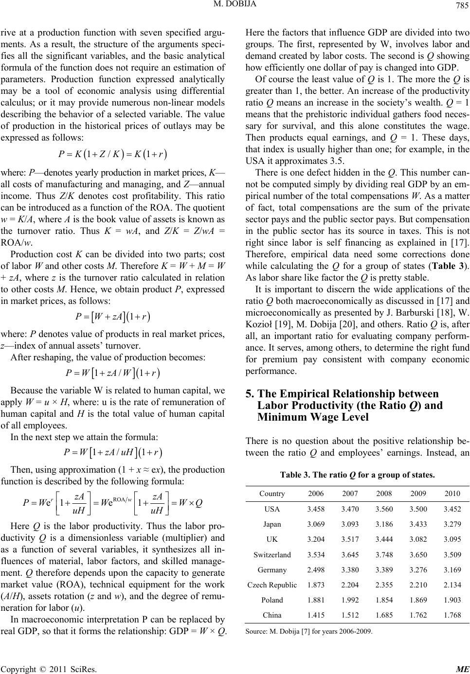 M. DOBIJA 785 rive at a production function with seven specified argu- ments. As a result, the structure of the arguments speci- fies all the significant variables, and the basic analytical formula of the function does not require an estimation of parameters. Production function expressed analytically may be a tool of economic analysis using differential calculus; or it may provide numerous non-linear models describing the behavior of a selected variable. The value of production in the historical prices of outlays may be expressed as follows: 1/ 1PKZK Kr where: P—denotes yearly production in market prices, K— all costs of manufacturing and managing, and Z—annual income. Thus Z/K denotes cost profitability. This ratio can be introduced as a function of the ROA. The quotient w = K/A, where A is the book value of assets is known as the turnover ratio. Thus K = wA, and Z/K = Z/wA = ROA/w. Production cost K can be divided into two parts; cost of labor W and other costs M. Therefore K = W + M = W + zA, where z is the turnover ratio calculated in relation to other costs M. Hence, we obtain product P, expressed in market prices, as follows: 1PWzA r where: P denotes value of products in real market prices, z—index of annual assets’ turnover. After reshaping, the value of production becomes: 1/1PW zAWr Because the variable W is related to human capital, we apply W = u × H, where: u is the rate of remuneration of human capital and H is the total value of human capital of all employees. In the next step we attain the formula: 1/ 1PW zAuHr Then, using approximation (1 + x ≈ ex), the production function is described by the following formula: ROA e1e 1 rw zA zA PW WWQ uH uH Here Q is the labor productivity. Thus the labor pro- ductivity Q is a dimensionless variable (multiplier) and as a function of several variables, it synthesizes all in- fluences of material, labor factors, and skilled manage- ment. Q therefore depends upon the capacity to generate market value (ROA), technical equipment for the work (A/H), assets rotation (z and w), and the degree of remu- neration for labor (u). In macroeconomic interpretation P can be replaced by real GDP, so that it forms the relationship: GDP = W × Q. Here the factors that influence GDP are divided into two groups. The first, represented by W, involves labor and demand created by labor costs. The second is Q showing how efficiently one dollar of pay is changed into GDP. Of course the least value of Q is 1. The more the Q is greater than 1, the better. An increase of the productivity ratio Q means an increase in the society’s wealth. Q = 1 means that the prehistoric individual gathers food neces- sary for survival, and this alone constitutes the wage. Then products equal earnings, and Q = 1. These days, that index is usually higher than one; for example, in the USA it approximates 3.5. There is one defect hidden in the Q. This number can- not be computed simply by dividing real GDP by an em- pirical number of the total compensations W. As a matter of fact, total compensations are the sum of the private sector pays and the public sector pays. But compensation in the public sector has its source in taxes. This is not right since labor is self financing as explained in [17]. Therefore, empirical data need some corrections done while calculating the Q for a group of states (Table 3). As labor share like factor the Q is pretty stable. It is important to discern the wide applications of the ratio Q both macroeconomically as discussed in [17] and microeconomically as presented by J. Barburski [18], W. Kozioł [19], M. Dobija [20], and others. Ratio Q is, after all, an important ratio for evaluating company perform- ance. It serves, among others, to determine the right fund for premium pay consistent with company economic performance. 5. The Empirical Relationship between Labor Productivity (the Ratio Q) and Minimum Wage Level There is no question about the positive relationship be- tween the ratio Q and employees’ earnings. Instead, an Table 3. The ratio Q for a group of states. Country 2006 2007 2008 2009 2010 USA 3.458 3.470 3.560 3.500 3.452 Japan 3.069 3.093 3.186 3.433 3.279 UK 3.204 3.517 3.444 3.082 3.095 Switzerland 3.534 3.645 3.748 3.650 3.509 Germany 2.498 3.380 3.389 3.276 3.169 Czech Republic1.873 2.204 2.355 2.210 2.134 Poland 1.881 1.992 1.854 1.869 1.903 China 1.415 1.512 1.685 1.762 1.768 Source: M. Dobija [7] for years 2006-2009. Copyright © 2011 SciRes. ME 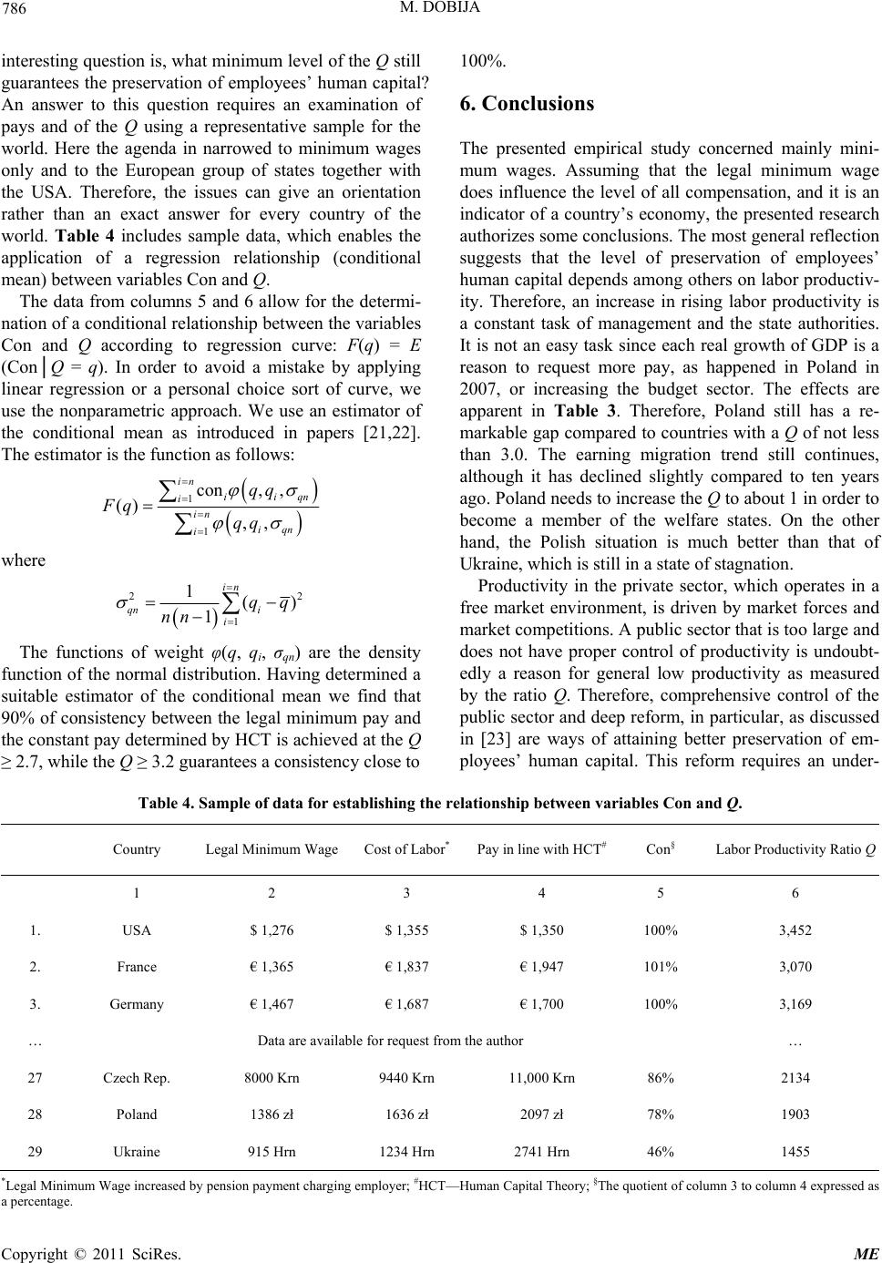 M. DOBIJA Copyright © 2011 SciRes. ME 786 interesting question is, what minimum level of the Q still guarantees the preservation of employees’ human capital? An answer to this question requires an examination of pays and of the Q using a representative sample for the world. Here the agenda in narrowed to minimum wages only and to the European group of states together with the USA. Therefore, the issues can give an orientation rather than an exact answer for every country of the world. Table 4 includes sample data, which enables the application of a regression relationship (conditional mean) between variables Con and Q. 100%. 6. Conclusions The presented empirical study concerned mainly mini- mum wages. Assuming that the legal minimum wage does influence the level of all compensation, and it is an indicator of a country’s economy, the presented research authorizes some conclusions. The most general reflection suggests that the level of preservation of employees’ human capital depends among others on labor productiv- ity. Therefore, an increase in rising labor productivity is a constant task of management and the state authorities. It is not an easy task since each real growth of GDP is a reason to request more pay, as happened in Poland in 2007, or increasing the budget sector. The effects are apparent in Table 3. Therefore, Poland still has a re- markable gap compared to countries with a Q of not less than 3.0. The earning migration trend still continues, although it has declined slightly compared to ten years ago. Poland needs to increase the Q to about 1 in order to become a member of the welfare states. On the other hand, the Polish situation is much better than that of Ukraine, which is still in a state of stagnation. The data from columns 5 and 6 allow for the determi- nation of a conditional relationship between the variables Con and Q according to regression curve: F(q) = E (Con│Q = q). In order to avoid a mistake by applying linear regression or a personal choice sort of curve, we use the nonparametric approach. We use an estimator of the conditional mean as introduced in papers [21,22]. The estimator is the function as follows: 1 1 con, , () ,, in iiq i in iqn i qq Fq qq n where 2 1 1() 1 in qn i i qq nn 2 Productivity in the private sector, which operates in a free market environment, is driven by market forces and market competitions. A public sector that is too large and does not have proper control of productivity is undoubt- edly a reason for general low productivity as measured by the ratio Q. Therefore, comprehensive control of the public sector and deep reform, in particular, as discussed in [23] are ways of attaining better preservation of em- ployees’ human capital. This reform requires an under- The functions of weight φ(q, qi, σqn) are the density function of the normal distribution. Having determined a suitable estimator of the conditional mean we find that 90% of consistency between the legal minimum pay and the constant pay determined by HCT is achieved at the Q ≥ 2.7, while the Q ≥ 3.2 guarantees a consistency close to Table 4. Sample of data for establishing the relationship between variables Con and Q. Country Legal Minimum Wage Cost of Labor* Pay in line with HCT#Con§ Labor Productivity Ratio Q 1 2 3 4 5 6 1. USA $ 1,276 $ 1,355 $ 1,350 100% 3,452 2. France € 1,365 € 1,837 € 1,947 101% 3,070 3. Germany € 1,467 € 1,687 € 1,700 100% 3,169 … Data are available for request from the author … 27 Czech Rep. 8000 Krn 9440 Krn 11,000 Krn 86% 2134 28 Poland 1386 zł 1636 zł 2097 zł 78% 1903 29 Ukraine 915 Hrn 1234 Hrn 2741 Hrn 46% 1455 *Legal Minimum Wage increased by pension payment charging employer; #HCT—Human Capital Theory; §The quotient of column 3 to column 4 expressed as percentage. a  787 M. DOBIJA standing and application of labor self-financing as well as a limitation of total pays in the public sector according to the size of the Q. We can conclude that labor produc- tivity measured by ratio Q is significant factor influence- ing level of the minimum wage. Nevertheless it is not exclusive factor. The mentioned Gini’s coefficient of earnings distribution as well the too large public sector are also essential factors. 7. References [1] M. Blaug, “The Methodology of Economics,” Wyda- wnictwo Naukowe PWN, Warsaw, 1955. [2] M. Dobija, “Abstract Nature of Capital and Money, in Linda M. Cornwall, New Developments in Banking and Finance,” Chapter 4, Nova Science Publishers, Inc., New York, 2007, pp. 89-114. [3] B. Kurek, “The risk premium estimation on the basis of adjusted ROA in I. Górowski, General Accounting The- ory,” Evolution and Design for Efficiency, Wydawnictwa Akademickie i Profesjonalne, Warsaw, 2008, pp. 375- 392. [4] B. Kurek, “Deterministic Risk Premium Hypothesis,” Wydawnictwo UEK, Kraków, 2010. [5] P. Atkins, “Galileeo’s Finger—The Ten Great Ideas of Science,” 2005. [6] M. Dobija, “Labor Productivity Ratio and International Comparison of Economic Performance—Formalization of the PPP Theory and Preliminary Examinations,” EMER-GO, No. 1/2008, 2008, pp. 3-19. [7] M. Dobija, “Abstract Nature of Money and the Modern Equation of Exchange,” Modern Economy, 2011, Vol. 2, May 2011, pp. 142-152. doi:10.4236/me.2011.20019 [8] E. Libanowa, “Demographic Collapse,” Official Journal, Vol. 40, 2004, p. 11. [9] M. Dobija, “Human Resources Costing and Accounting as a Determinant of Minimum Wage Theory,” Zeszyty Naukowe UEK, Vol. 553, 2000, pp. 39-61. [10] W. Kozioł, “Human Capital as Foundation for Shaping of Constant Pay,” In: M. Dobija, Theory of Measurement of Capital and Profit, Wydawnictwo UEK, Kraków, 2010, pp. 73-100. [11] J. Renkas, “Analysis of Minimal Wage in Ukraine Using Human Capital Theory,” Proceedings of conference ІХ-ї міжнаро- дної наукової конференції; Житомир, 2010, pp. 195-199. [12] J. Barburski, “Premium Pay as a Function of Labor Productivity,” In: M. Dobija, Theory of Measurement of Capital and Profit, Wydawnictwo UEK, Kraków, 1982, pp. 101-117. [13] I. Cieślak, “Value of Human Capital and Wage Dispari- ties in I. Górowski, General Accounting Theory,” Evolution and Design for Efficiency, Wydawnictwa Akademickie i Profesjonalne, Warsaw, 2008, pp. 289-303. [14] S. Sunder, “Theory of Accounting and Control,” South-Western Publishing, Cincinnati, 1997. [15] M. Dobija, “Analytic Production Function,” Ekonomika i Organizacja Przedsię-Biorstwa, Vol. 658, No. 11, 2004, pp. 9-17. [16] M. Dobija, “Labor Productivity Ratio and International Comparison of Economic Performance—Formalization of the PPP Theory and Preliminary Examinations,” EMER-GO, No. 1/2008, 2008, pp. 3-19. [17] M. Dobija, “Abstract Nature of Money and the Modern Equation of Exchange,” Modern Economy, Vol. 2, 2011, pp. 142-152. doi:10.4236/me.2011.20019 [18] J. Barburski, “Premium pay as a function of labor productivity,” In: M. Dobija, Theory of Measurement of Capital and Profit, Wydawnictwo UEK, Kraków, 1982, pp. 101-117. [19] W. Kozioł, “Production Function in Shaping of Compen- sations,” Zeszyty Naukowe UEK, Vol. 752, 2007, pp. 125- 136. [20] M. Dobija, “Analytic Production Function,” Ekonomika i Organizacja Przedsię-Biorstwa, Vol. 658, No. 11, 2004, pp. 9-17. [21] M. Dobija, “Analytic Distribution Function,” Przegląd Statystyczny, Vol. 29, No. 1, 1982, pp. 207-220. [22] E. Smaga and M. Dobija, “Some Application of Non-Parametric Regression Estimators,” Przegląd Staty- styczny, Vol. 34, No. 1, 1987, pp. 19-28. [23] M. Dobija, “Abstract Nature of Money and the Modern Equation of Exchange,” Modern Economy, Vol. 2, May 2011, pp. 142-152. doi:10.4236/me.2011.20019 Copyright © 2011 SciRes. ME
|