Modern Economy, 2011, 2, 735-742
doi:10.4236/me.2011.25082 Published Online November 2011 (http://www.SciRP.org/journal/me)
Copyright © 2011 SciRes. ME
735
Speed of Adjustment and Infraday/Intraday Volatility in
the Italian Stock and Futures Markets
Pietro Gottardo
Dipartimento di Ricerche Aziendali, Facoltà di Economia, Pavia, Italy
E-mail: pgottardo@eco.unipv.it
Received July 15, 201 1; revised August 19, 2011; accepted September 1, 201 1
Abstract
We estimate the speed of adjustment of prices to value changes in the Italian stock and futures markets using
variances in different return intervals. The paper presents evidence that an assumption of linearity for the
relationship volatility-time is untenable when intraday and infraday data are used jointly. Prices adjust to
new information within three days, but the process is complex with evidence of overshooting and divergent
movements in the smaller return intervals. Firms behave differently according to their inclusion or exclusion
from the MIB30 index. The speed of adjustment is strongly related to firm-specific characteristics and the
log of capitalization explains some of the cross-sectional variability in the adjustment coefficients for most of
the return intervals.
Keywords: Speed of Adjustment, Overshooting, Intraday returns, Stock Index Future
1. Introduction
The growing body of evidence on stock returns predict-
ability and overreaction challenges the traditional effi-
ciency view that stock prices reflect fully and quickly all
the relevant information. Event-based return predictabil-
ity, long term reversals and short term momentum, ex-
cessive stock prices volatility relative to fundamentals
are some of the findings of a large number of empirical
works in different areas, countries and time periods.
Daniel-Hirshleifer and Subrahmanyam [1] cite a large
sample of the relevant literature on these topics.
There is disagreement over the interpretation of this
evidence. The anomalies may be considered normal
chance deviations from the fundamental efficiency law
as suggested by Fama [2], but the regularity and dimen-
sion of these phenomena cast some doubt on the appro-
priateness of this hypothesis. An alternative explanation
is that many empirical regularities represent variations in
rational risk premia, even if this requires an asset pricing
model with extreme variability in marginal utility across
states and has other undesirable implications.
Daniel-Hirshleifer and Subrahmanyam [1] suggest a
psychological model based on imperfect rationality, in
particular they construct their model on two well-known
psychological biases: investor overconfidence about the
precision of his private information, and biased self-at-
tribution which causes individuals to strongly attribute
events that confirm the validity of their actions to high
ability and events that disconfirm the action to external
noise or sabotage.
Another stream of literature suggests instead a lagged
adjustment of security prices to new information. Patell-
Wolfson [3] and Hasbrouck-Ho [4] are just two exam-
ples of empirical studies showing that prices tak e time to
adjust to news. Patell-Wolfson [3] examine intraday
price changes associated with earnings announcements.
From a theoretical perspective the derivation of a partial
price adjustment model in security markets, showing that
this is the result of optimizing behavior by market mak-
ers is due to Garbade-Silber [5,6]. Goldman-Beja [7],
Amihud-Mendelson [8], and Damodaran [9] describe a
return process that can be applied to portfolios and ind ex
futures as well as single stocks which permits the deriva-
tion of a measure for the price adjustment coefficient.
The model derived in Amihud-Mendelson [8] and in
Damodaran [9] distinguishes between observed prices
and intrinsic value of a stock, measuring a finite speed of
adjustment of prices to value changes using the informa-
tion in various return intervals.
The screening among all these models is just an em-
pirical matter, only the real behavior of prices in security
markets can shed some light on the subject. In what fol-
lows we use Damodaran adjustment model in the correct
P. GOTTARDO
736
form derived by Brisley-Theobald [10], with a signifi-
cant difference in h is assumption with resp ect to the rela-
tionship between time and v olatility, to analyze the price
adjustment in the Italian futures and stock markets. The
primary contribution of this paper is a refinement of the
model in Damodaran [9] to account for the estimation of
adjustment coefficients using together intraday and in-
fradaily data and its application to a new data-set to dis-
entangle the relative merits of the above models. We
calculate returns and variances over non-overlapping
periods and estimate the price adjustment coefficients at
intraday intervals of five, fifteen, thirty, sixty minutes,
two, four, and eight hours and at infraday frequencies
from one to ten days. The relationship between time and
volatility is a key empirical problem, usually solved as-
suming the linearity of this relationship. Using on ly daily
returns a linear approximation could be reasonable but
not with the inclusion of in traday returns. As we show in
section 3 the inclusion of both infraday and intraday
measurement intervals has a severe impact on the linear-
ity of the relationship, so that the usual assumption is
untenable using datasets and models that take into ac-
count jointly information on the volatility within a trad-
ing day (intraday intervals) and across trading days (in-
fraday interv als). Section 2 presents the price adjustment
model used. We analyze in section 3 the return behavior
of the Italian stock index and stock index futures together
with a selection of single stocks. The choice is useful to
screen possible differential adjustment processes for the
index, futures and the single securities as half of this
sample is given by stocks not included in the index over
which the futures contract is designed. Section 4 con-
cludes with a discussion of our results and some policy
implications about the efficiency and liquidity improve-
ment of the assets negotiated in these markets.
2. Price-Adjustment Model
The price adjustment model of Amihud and Mendelson
[8] distinguishes between the intrinsic value of a stock,
futures or portfolio, Vt, and the observed price, Pt.
A generalization of their interpretation of this model
allows for market-related, specific information and noise
to be reflected in the return process, resulting in an im-
perfect (partial or lagged) price adjustments to value
changes, but also for overshooting phenomena (a more-
than-perfect adjustment) or divergence from value. The
basic model is
,,1,,1 ,
it itit itit
P
PgVP u


 

(1)
where g represents the speed of price adjustment: g = 1
implies a full and almost immediate (as the one period
lag can be small as you like) adjustment of prices to
every change in value, g > 1 represents a tendency for
the asset to overreact to news affecting its value, whereas
0 < g < 1 includes all cases of partial and lagged adjust-
ment. Last but not least for importance is the case when
g < 0 that implies price divergence from the intrinsic
value.
The possibilities of overreaction or divergence from
value have been totally neglected in the theoretical de-
velopments of this model by Amihud-Mendelson [8] and
Damodaran [9] but given the results in DeBondt-Thaler
[11] and the implications of behavioral or psychological
models for the price generation process we believe that a
careful investigation is called for. The noise term, ui,t in
Equation (1) is determined by information and markets
structure related factors such as liquidity trading, noise,
bid-ask spread. It is assumed to be a sequence of i.i.d.
random variables with zero mean and finite variance, σ2i
and independent across stocks.
To derive a measure of g, Damodaran [9] uses the
variances in different return intervals that can be written
as

,2
,,,
2
Var 22
ij
ijt
ij ij
g
Rjv
gg
2


(2)
where Var(Ri,jt) is the variance for the observed returns
assuming j as measurement interval, while gj is the ad-
justment coefficient measured for the same j-interval
returns, and v2 is the variance of the intrinsic value proc-
ess.
A restrictive by-product of the original assumptions of
this model is that v2 is linear in j, as {Vt} is an i.i.d. ran-
dom variable and the intrinsic variance and noise proc-
esses are assumed to be independent. This assumption is
apparently innocuous given that a linear relationship
between volatility and calendar time is almost standard
in many areas of research in finance. Unfortunately even
with daily data it is a well known and established result
that a linear relation between volatility and time is at best
a first approximation as weekends and other non-work-
ing holidays have a less than proportional effect on stock
volatility. The problem is of great concern here because
our intention is to measure the price adjustment coeffi-
cients using together intraday and infradaily data, see for
instance Amihud-Mendelson [12], Amihud-Mendelson
and Murgia [13], and Gottardo [14]. To the degree that
this hypothesis is violated, the model estimates of gj will
be grossly flawed. We suggest to replace Equation (2)
with the following more general formulation:

,2
,,,
2
Var()
22
ij
ijt
ij ij
g
Rfjv
gg
2


(2’)
analyzing three different forms for the relationship be-
Copyright © 2011 SciRes. ME
P. GOTTARDO
Copyright © 2011 SciRes. ME
737
tween intrinsic volatility and return measurement inter-val:
1
() 1 and 1 for 1 1 for
empirical average relation between t ime and volatility
jjk
fj jdj kdjldlj k

 
The first one is the usual assumption of linearity in
variance while the second form give us some freedom
particularly u seful if we choose the poin t of discontinu ity
l of this relationship to represent the passage from intra-
day to infraday return intervals.
With the third formulation we relay on the data to de-
termine without theoretical constraints what is the em-
pirical law characterizing the volatility evolution through
measurement intervals.
We can now use a sequence of n observed unit-inter-
val returns to estimate the variances for different return
intervals (j = 1, 2,, k) and assume that this sequence is
of sufficient length to allow gk = 1. Given Equation (2’)
we can then derive the price adjustment coefficients gj if
we impose some structure for the noise and intrinsic
variance components.
The assumption in Damodaran [9] was that the two
components could be written as functions of the covari-
ance and variance in k-interval returns. But this is just a
matter of convenience, the model offers no theoretical
support for this choice. We retain only partially this hy-
pothesis assuming the intrinsic variance to be function of
the k-interval variance while the noise component de-
pends from all the auto-covariances in the infraday return
intervals. The reason is that while the choice of the k-
interval variance is innocuous and easily in terchangeable
given a clear association between volatility and time, this
is untrue for the covariances that change in a manner
unpredictable through time with large swings even from
positive to negative values and vice-versa. Using the
average auto-covariance over all infraday intervals we
minimize the effect on the results obtaining more stable
gj’s estimates. Writing the noise and intrinsic variance
components as

2,,1
Cov ,
iijtijt
ljkRR
 (3)
,,
2Var() 2Cov,
ikti jti jt
RRR
vk
,1
(4)
On the base of Equation (2’) we can calculate for each in-
terval j, the difference between the variance in j-interval
returns and the equivalent variance in k-interval returns.
Substituting for v2 and σ2 and solving through for gj, we get
Equation (5).
In theory (5) could be used to estimate the speed of
adjustment for return intervals until j = k – 1, with only
the information available in the time series of unit-in-
terval returns data. In practice given that unit-interval
returns of intraday frequency do not contain information
with respect to the overnight returns we need an addi-
tional data source that could be represented by the daily
stock returns.
3. Estimation and Results
3.1. Data Sample and Methodological Choices
To estimate the speed of price adjustment, we use 5 min-
utes as unit-interval from July 4, 1995 to May 30, 1997.
The sample includes the index of the 30 most important
Italian stocks (MIB30), the futures contract on this index
(FIB30), all the firms included in the MIB30 (for the
whole sample period or partially) as well as the biggest
firms not included in this index. The final sample is
composed of 58 stocks listed on the Italian Stock Ex-
change.
The primary reason for the sample size and the crite-
rion for inclusion was the availability of data combined
with enough liquidity for each stock. We use all returns
from opening to close (10 a.m. to 17 p.m. for the stock
market and 9.30 a.m. 17.30 p.m. for the futures market)
and the daily returns to estimate for each stock, the index
and the futures, the variances with return frequencies
ranging from five minutes to ten days.
We calculate returns and variances over non-overlap-
ping periods and estimate the price adjustment coeffi-
cients at intervals of five, fifteen, thirty, sixty minutes,
two, four, and eight hours and at daily frequencies from
one to ten days. The first empirical problem to solve is
related to the relationship between time and volatility.
Using only daily returns a linear approximation could be
reasonable but not with the inclusion of intraday returns.
The plot in the Figure 1 below shows the average
stock volatility for the intraday return intervals. As can
be seen a linear relationship is acceptable as a first ap-
proximation only for the intervals between two and eight

,,,1
,
,,,,
2Var() Cov,()
Var()( )Var()2Cov,
ijtijtijt
ij
ijtiktijtijt
RfjRR fj
g
RfjRkRR k



 1
(5)
P. GOTTARDO
738
hours, the inclusion of smaller or greater measurement
intervals (as the daily interval with its overnight effect)
has a severe impact on the linearity of the relationship.
Three other figures not included here but available
upon request show the empirical relation that exists be-
tween volatility and measurement interval for the futures,
the stock index and the single stocks. In this last case the
average empirical law as been estimated using the ob-
served variances for each stock in every return interval.
The conclusion is that a linear relationship does a good
job for return intervals ranging from one to nine days and
perhaps in some intraday range for the futures and the
stock index but overall it is a poor approximation of the
true relation that seems to exist between time and volatil-
ity. This result is particularly true looking at single
stocks.
3.2. Adjustment Coefficients Estimates
To measure the impact of this methodological choice
on the adjustment coefficients we present three series of
results using: a) a linear relation between intrinsic vari-
ance and time; b) a linear relation but with a flat step
going from the eight-hours to one-day return intervals; c)
the empirical relationships. The cross-sectional average
of the adjustment coefficients for all stocks in our sample,
as well as the coefficients for the index and index futures
are reported in Table 1.
From the results we can draw some interesting obser-
vations. First, there seems that the form of the relation
ship time-volatility has a strong effect on the estimates,
even if as could be expected the differences between the
three sets of results decay exponentially and are almost
zero after the eight hours interval. Second, the adjust-
ment coefficients estimated for the index and the futures
contract suggest strong overshooting effects over the
smaller measurement intervals that only after three days
(four days for the index) of continuous trading are reab-
sorbed. This finding is consistent with herding behavior
and psychological overshooting models. Third, the aver-
age cross-sectional coefficients for the 58 stocks displays
even more interesting properties, as they suggest diver-
Figure 1. Average volatility for 58 securities in the intra-
day return intervals. Period 1995:7-1997:5.
Table 1. Speed of price adjustment: 1995/7 to 1997/5. Cross sectional averages, index and index futures coefficients for seven-
teen return intervals ranging from five minutes to ten days.
Interval stocks mib30 fib30 stocks mib30 fib30 stocks mib30 fib30
5’ –9.9376 25.4676 15.525 –8.0501 15.2178 8.8659 –4.2434 18.9577 12.3483
15’ –3.6171 9.6901 6.0333 –2.8442 5.6918 3.436 –1.7994 7.374 4.8174
30’ –1.6365 5.3059 3.612 –1.2941 3.1873 2.0716 –1.016 3.9234 2.8557
1 hour –0.4495 3.3333 2.4242 –0.3915 1.9947 1.4041 –0.3672 2.4766 1.8909
2 hours 0.386 2.3333 1.854 0.1917 1.3926 1.0894 0.2101 1.7395 1.4186
4 hours 0.8697 1.8284 1.5957 0.5344 1.09 0.9559 0.6078 1.365 1.1912
8 hours 1.1559 1.589 1.4927 0.7374 0.9596 0.9144 0.8459 1.1673 1.0843
1 day 0.8537 0.9623 0.9413 0.8537 0.9623 0.9413 0.8732 1.1662 1.0791
2 days 0.9572 0.9135 0.8824 0.9572 0.9135 0.8824 0.9644 1.072 1.0382
3 days 0.9999 0.9192 0.8936 0.9999 0.9192 0.8936 0.9862 1.0403 1.0218
4 days 0.9817 0.9253 0.9096 0.9817 0.9253 0.9096 0.9956 1.0257 1.0137
5 days 0.9942 0.8835 0.906 0.9942 0.8835 0.906 0.9953 1.0203 1.0097
6 days 1.0377 0.8613 0.8312 1.0377 0.8613 0.8312 1.0182 1.0158 1.0091
7 days 1.0357 0.8662 0.8456 1.0357 0.8662 0.8456 1.0188 1.0114 1.0064
8 days 1.0211 0.9059 0.8885 1.0211 0.9059 0.8885 1.0139 1.0066 1.0038
9 days 1.0465 0.9514 0.9519 1.0465 0.9514 0.9519 1.0003 1.0029 1.0015
10 days 1 1 1 1 1 1 1 1 1
Copyright © 2011 SciRes. ME
P. GOTTARDO 739
gent movements from value within 60 minutes docu-
mented by negative values for the price adjustment coef-
ficients. For intervals of more than one hour there is a
lagged process of incorporation of the new information
in the stock prices and the average coefficient is positive,
going from 0.210 in the 60 minutes interval to 0.986 for
the three-day returns. Last, in all cases the adjustment of
security prices is almost completed between three and
five days of trading, this is true for the index and the fu-
tures but also for every single stock.
The results in Table 1 are consistent with a market
that adjusts slowly to new information, in agreement
with the findings in Damodaran [9], Patell-Wolfson [3],
and Hasbrouck-Lo [4] even if the adjustment process is
not “linear”, as it may result in very short term over-
shooting and divergence from equilibrium. Very short
here refers to periods on the order of five minutes to few
hours of trading. What about individual firms? Given
that the speed of adjustment is a function of market-wide
and firm-specific information, we should find significant
differences among stocks related for instance to the in-
clusion of a stock in the index, as it is likely that the fu-
tures trading has significant feedback effects on the stock
market, cfr. Tang [15] and Tang-Lui [16]. Size can also
be important, but as the single stocks are included in the
MIB30 on the base of size and trading the effect of this
variable could be intermingled with the previous one. A
similar conclusion is possible for other measures of the
quality and amount of information as volume of trading
or other liquidity proxies. A graphic analysis non in-
cluded here shows the dispersion across securities and
through return intervals for the estimated adjustment
coefficients. We see a rapid incorporation of new infor-
mation in prices for all stocks but it is noteworthy that
the variability in the speed of adjustment is higher as the
measurement interval is lessened. But a careful analysis
of the results shows that there are significant regularities
in the coefficients. Average adjustment coefficients for
firms classified as included for the entire sample period,
never included or partially included in the index of the
30 most important Italian stocks (MIB30) show that the
inclusion in the index seems to be a relevant factor in-
fluencing the measured adjustment coefficients. The
MIB30 stocks display the strongest movements away
from value up to intervals of two hours, while the ad-
justment of the no-index stocks is almost zero in the five
minutes interval but after that converges quickly to one.
For the stocks included in the index the price adjustment
is only 21 percent after four hours, and reaches the 80
percent only after one day of trading. This finding may
seem a bit surprising but we should remember two facts.
The first one, is that the higher liquidity induced also by
the trading in the futures contract increases the volatility
in the underlying stocks. The gain in efficiency related to
the creation of a futures contract has to be paid in some
way. A complete psychological model of price formation
should account for trial and error in the trading process
and learning as prices incorporate new information to
reach their underlying value. This is likely to be reflected
primarily in the prices of the most liquid stocks where is
concentrated the activity of traders and analysts. Second,
the nontrading has subtle effects on the way single stock
prices adjust to value. The trading in the biggest stocks is
really continuous while it is a step process for the other
stocks for well known reasons re lated to liquidity, cost of
trading, interest of institutional and other traders as well
as analysts following. The smaller stocks and, in general,
the stocks not included in an index underlying a futures
contract are then likely to be “followers”, i.e. stocks that
incorporate new information after the fact. This does not
necessarily imply that their price has a slower speed of
adjustment with respect to the big stocks, paradoxically
the high transaction costs (bid-ask spread and price im-
pact of trading) and a low liquidity may result in a
speedy adjustment process. What we mean is that the
cost of errors is too high in a small stock transaction and
(unless we are talking about a piece of firm-specific in-
formation), this induces the traders to concentrate their
activity on the stock index futures or in the liquid under-
lying stocks. In these two market segments the costs are
low, the liquidity is high and there is plenty of room for
learning and reverse a trade in case of errors (overshoot-
ing or misinterpretation of a piece of information). This
could explain why the firms not included in the MIB30
seem to adjust more quickly in the intraday intervals and
why the big stocks display some evidence of movements
away from equilibrium for intervals up to two hours.
3.3. Results on Speed of Adjustment and Firm
Characteristics
The results thus far are consistent with individual stocks
adjusting to market-wide and firm-specific news on the
base of characteristics as liquidity, size, inclusion in the
index underlying a futures, trading intensity and volume
of trading. To substantiate this hypothesis we present in
Table 2 the parameter estimates from regressions relat-
ing price adjustment coefficients and firm-specific fac-
tors. The proxy for size is represented from the log of
capitalization at the end of our sample period, the vol-
ume of trading is simply the average value of transac-
tions in every five-minutes interval for each single stock.
We measure the intensity in the trading process as the
percent of five-minutes intervals with a recorded transac-
tion in that stock. A dummy (D30) captures the effect of
inclusion in the MIB30, while another dummy, BIG6,
Copyright © 2011 SciRes. ME
P. GOTTARDO
740
Table 2. Price adjustment coe ffic ients and individual stocks characteristics. (a) Results for the relationship between 5-minute s
adjustment coefficients and firm specific factors such as the log of capitalization, trading intensity (% of unit-intervals with a
recorded transaction), volume of trading (average value of transactions in a unit-interval) and inclusion in the MIB30. T-stats
are in parenthesis; (b) Results for the relationship between the individual stocks speed of adjustment and firm size measured
as the log of capitalization in mid 1997 in every return interval from 5 minutes to 9 days.
(a)
Model Intercept Size Trading intensity Volume of trading D30 BIG6 Adj. R2
1 35.33** (3.08) –4.81** (–3.49) 0.16
2 3.69 (0.91) –14.63* (–2.16) 0.06
3 –2.70 (–1.34) –0. 15 ( –1. 44) 0.02
4 34.86* (2.41) –4.74* (–2.50) –0.24 (–0.05) 0.15
5 40.81** (2.85) –5.91** (–2.69) 6.55 (0.65) 0.15
6 56.16** (3.80) –7.53** (–4.08) 14.79* ( 2.14) 0.21
(b)
Return interval Intercept Size Adj. R2
5’ 35.33** (3.08) –4.813** (–3.49) 0.16
15’ 19.82** (3.27) –2.630** (–3.60) 0.17
30’ 14.90** (3.34) –1.936** (–3.60) 0.17
1 hour 10.70** (3.45) –1.346** (–3.60) 0.17
2 hours 7.07** (3.69) –0.834** (–3.62) 0.17
4 hours 4.25** (4.24) –0.443** (–3.67) 0.18
8 hours 2.57** (5.46) –0.210** (–3.70) 0.18
1 day 1.84** (4.78) –0.118* (–2.54) 0.09
2 days 1.28** (8.08) –0.039* (–2.03) 0.05
3 days 1.07** (8.87) –0.010 (–0.71) 0
4 days 0.97** (8.98) 0.003 (0.21) 0
5 days 0.89** (10.14) 0.013 (1.22) 0.01
6 days 0.78** (7.30) 0.029* (2.24) 0.07
7 days 0.73** (7.42) 0.035** (2.96) 0.12
8 days 0.78** (7.66) 0.028* (2.26) 0.07
9 days 0.83** (6.66) 0.021 (1.43) 0.02
Superscripts **, *, and represent significance at the 1%, 5% and 10 % level.
singles out the six biggest Italian stocks (Generali, Fiat,
Telecom, Eni, Tim, Stet).
Table 2(a) shows the results with the five-minutes
adjustment coefficients as dependent variable. The vol-
ume of trading per se seems unrelated to the speed of
adjustment in the unit-interval, while the effect of the
variable measuring trading intensity becomes not sig-
nificant when we add size to the regression. This is
probably due to the positive correlation existing between
size and this variable. Size is always significant and its
beta is negative so that an increase in size is associated
with a reduction in the adjustment coefficient. In terms
of unit-interval gi’s this implies more cases of over-
shooting between small stocks and an increase in the
frequency of divergent movements as size grows.
The dummy for inclusion in the MIB30 is not signifi-
cant when we control for size but the dummy for the six
most important stocks retains its significance and this has
the effect of reversing the impact of size on the adjust-
ment coefficient for high levels of capitalization.
Table 2(b) presents the regression results for the rela-
tionship between speed of adjustment and stock size in
each return interval. The results in Table 2(b) confirm
that firm size is strongly related to the measured speed of
adjustment.
The relationship between adjustment coefficients and
the log of capitalization is consistently negative for
measurement intervals ranging from five minutes to three
days and statistically significant but for the last interval.
The direction of this relationship is reversed for return
intervals of four days or more, but in this case size is
significant only for the intervals from six to eight days.
The results presented in Table 2 are based on the ad-
justment coefficients estimated using the empirical rela-
tionship between time and volatility but qualitatively the
results are the same even if we use the other two forms
Copyright © 2011 SciRes. ME
P. GOTTARDO 741
of the relationship.
Overall our results support the proposition that stock
prices adjust slowly to new information but in a different
manner for small and big firms and this is reflected in a
highly significant relation between adjustment coeffi-
cients and stock size. The inclusion in the MIB30 index
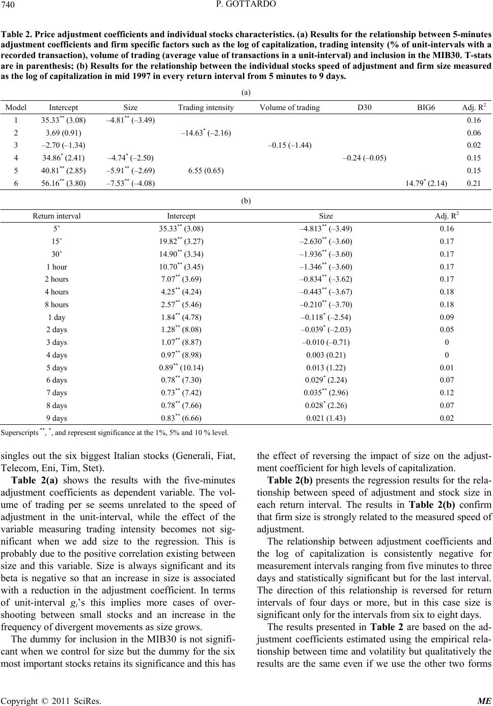
does not seem to be a relevant factor but this is the result
of two facts. First, only the biggest stocks are included in
the index, adding size as explanatory variable is likely to
dim any effect related to a dummy controlling for the
participation in the index. Second, among the big firms
the trading is highly concentrated in few stocks and is
not by chance that in Table 2(a) a dummy like BIG6 is
significant even when the MIB30 dummy is added to
model 6 (not shown). These six stocks are the core of
every portfolio whose aim is to replicate the index and
are necessary to implement any strategy requiring trading
in the futures and the unde rl ying m a rk et .
4. Conclusions
The degree of efficiency in the stock and futures markets
can be measured by the speed with which prices adjust to
incorporate new information. This process may be slow
with prices that take time to reflect value changes or very
speedy. It is also possible that in very short intervals or
in the long period prices display patterns that lead away
from equilibrium (at least temporarily) or give rise to
under and ov erreaction phenomen a.
This paper adapts the model developed in Amihud-
Mendelson [8] and Damodaran [9] to consider jointly
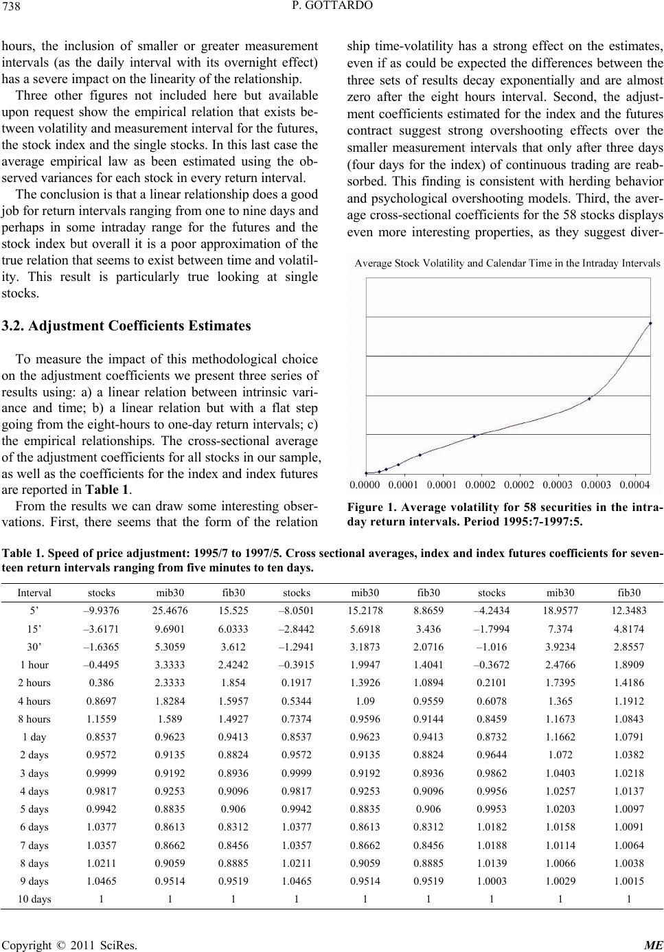
intraday and infraday data. The speed of adjustment is
estimated as function of the variances in different return
intervals from five minutes to ten days, as well as the
covariances in the infraday intervals. The approach is
then applied to the Italian index (MIB30) and index fu-
tures (FIB30), and to a sample of the most important
stocks listed in this market.
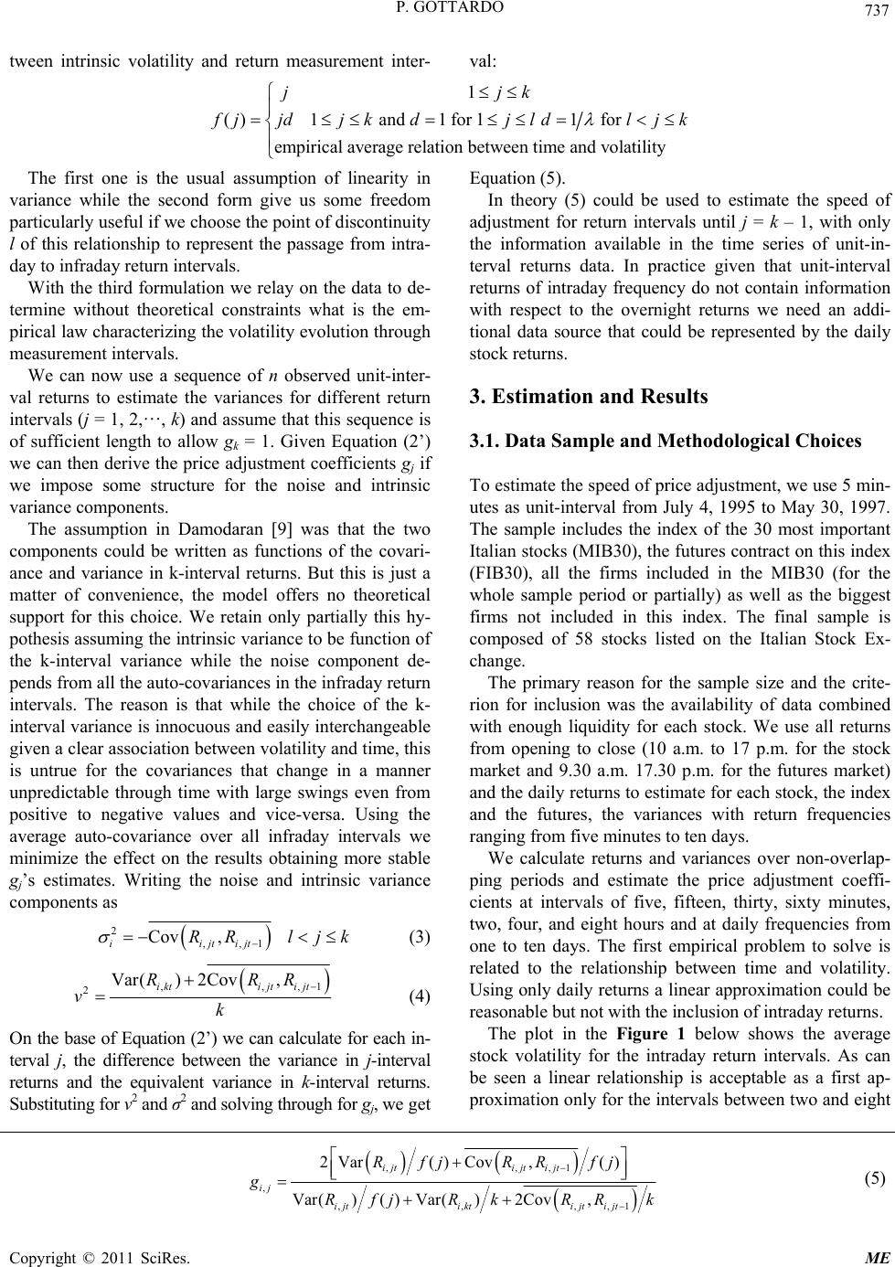
We show that the assumptions about the form of the
relationship between return volatility and time are critical
for the measured adjustment coefficients, the hypothesis
of linearity cannot be accepted using jointly intraday and
infraday returns as the resulting estimates are grossly
inflated for the smaller measurement intervals. We find
evidence that prices adjust slowly to new information,
three to five days of trading are necessary to complete
the adjustment and this is true for the index futures but
also on average for each individual stock. We also find
evidence that there is no simple intraday adjustment
process, the futures seems to overreact for small return
intervals, while on average the individual stocks diverge
from value for intervals up to two hours and then show a
pattern of lagged adjustment.
There are peculiar regularities in the price adjustment
of single stocks and the firms included in the index un-
derlying the futures behave differently from the others.
The analysis of the relationship between adjustment co-
efficients and firm characteristics confirms that size is
strongly related to the measured speed of adjustment for
most of the measurement intervals
5. References
[1] K. Daniel, D. Hirshleifer and A. Subrahmanyam, “Inves-
tor Psychology and Security Market Under- and Overre-
actions,” Journal of Finance, Vol. 53, No. 6, 1998, pp.
1839-1885. doi:10.1111/0022-1082.00077
[2] E. F. Fama, “Market Efficiency, Long Term Returns and
Behavioral Finance,” Journal of Financial Economics,
Vol. 49, No. 3, 1998, pp. 283-306.
doi:10.1016/S0304-405X(98)00026-9
[3] J. M. Patell and M. A. Wolfson, “The Intraday Speed of
Price Adjustment of Stock Prices to Earnings and Divi-
dend Announcements,” Journal of Financial Economics,
Vol. 13, No. 2, 1984, pp. 223-252.
doi:10.1016/0304-405X(84)90024-2
[4] J. Hasbrouck and T. Ho, “Order Arrival, Quote Behavior
and the Return-Generating Process,” Journal of Finance,
Vol. 42, No. 4, 1987, pp. 1035-1049.
doi:10.2307/2328305
[5] K. Garbade and W. Silber, “Structural Organization of
Secondary Markets: Clearing Frequency, Dealer Activity
and Liquidity Risk,” Journal of Finance, Vol. 34, No. 3,
1979, pp. 577-593. doi:10.2307/2327427
[6] K. Garbade and W. Silber, “Price Movement and Price
Discovery in Futures and Cash Markets,” Review of
Economics and Statistics, Vol. 65, No. 2, 1983, pp. 289-
297. doi:10.2307/1924495
[7] B. Goldman and A. Beja, “Market Prices vs. Equilibrium
Pri ces: Return’s Variance, Serial Correlation, and the Role
of the Specialist,” Journal of Finance, Vol. 34, No. 3,
1979, pp. 595-607. doi:10.2307/2327428
[8] Y. Amihud, and H. Mendelson, “Index and Index-Futures
Returns,” Journal of Accounting, Auditing & Finance,
Vol. 4, No. 2, 1989, pp. 415-431.
[9] A. Damodaran, “A Simple Measure of Price Adjustment
Coefficients,” Journal of Finance, Vol. 48, No. 1, 1993,
pp. 387-400. doi:10.2307/2328896
[10] N. Brisley and M. Theobald, “A Simple Measure of Price
Adjustment Coefficients: A Correction,” Journal of Fi-
nance, Vol. 51, No. 1, 1996, pp. 381-382.
doi:10.2307/2329314
[11] W. F. M. DeBondt and R. H. Thaler, “Does the Stock
Market Overreact?” Journal of Finance, Vol. 40, No. 3,
1985, pp. 793-808. doi:10.2307/2327804
[12] Y. Amihud and H. Mendelson, “Trading Mechanisms and
Stock Returns: An Empirical Investigation,” Journal of
Finance, Vol. 42, No. 3, 1987, pp. 533-553.
doi:10.2307/2328369
Copyright © 2011 SciRes. ME
P. GOTTARDO
Copyright © 2011 SciRes. ME
742
[13] Y. Amihud, H. Mendelson and M. Murgia, “Stock Mar-
ket Microstructure and Return Volatility: Evidence from
Italy,” Journal of Banking and Finance, Vol. 14, No. 2-3,
1990, pp. 423-440. doi:10.1016/0378-4266(90)90057-9
[14] P. Gottardo, “Dinamica dei Rendimenti e relazioni lead-
lag fra il FIB30 e l’indice MIB30,” Studi e Note di Eco-
nomia, Vol. 3, No. 3, 1998, pp. 69-103.
[15] G. Y. N. Tang, “Return Volatilities of Stock Index Fu-
tures in Hong Kong: Trading vs Non-Trading Periods,”
Journal of Derivatives, Vol. 4, No. 1, 1996, pp. 55-62.
doi:10.3905/jod.1996.407961
[16] G. Y. N. Tang and D. T. W. Lui, “Intraday and Intraweek
Volatility Patterns of Hang Seng Index and Index Futures,
and a Test of the Wait-To-Trade Hypothesis,” Pacific-
Basin Finance Journal, Vol. 10, No. 4, 2002, pp. 475-495.
doi:10.1016/S0927-538X(02)00069-0