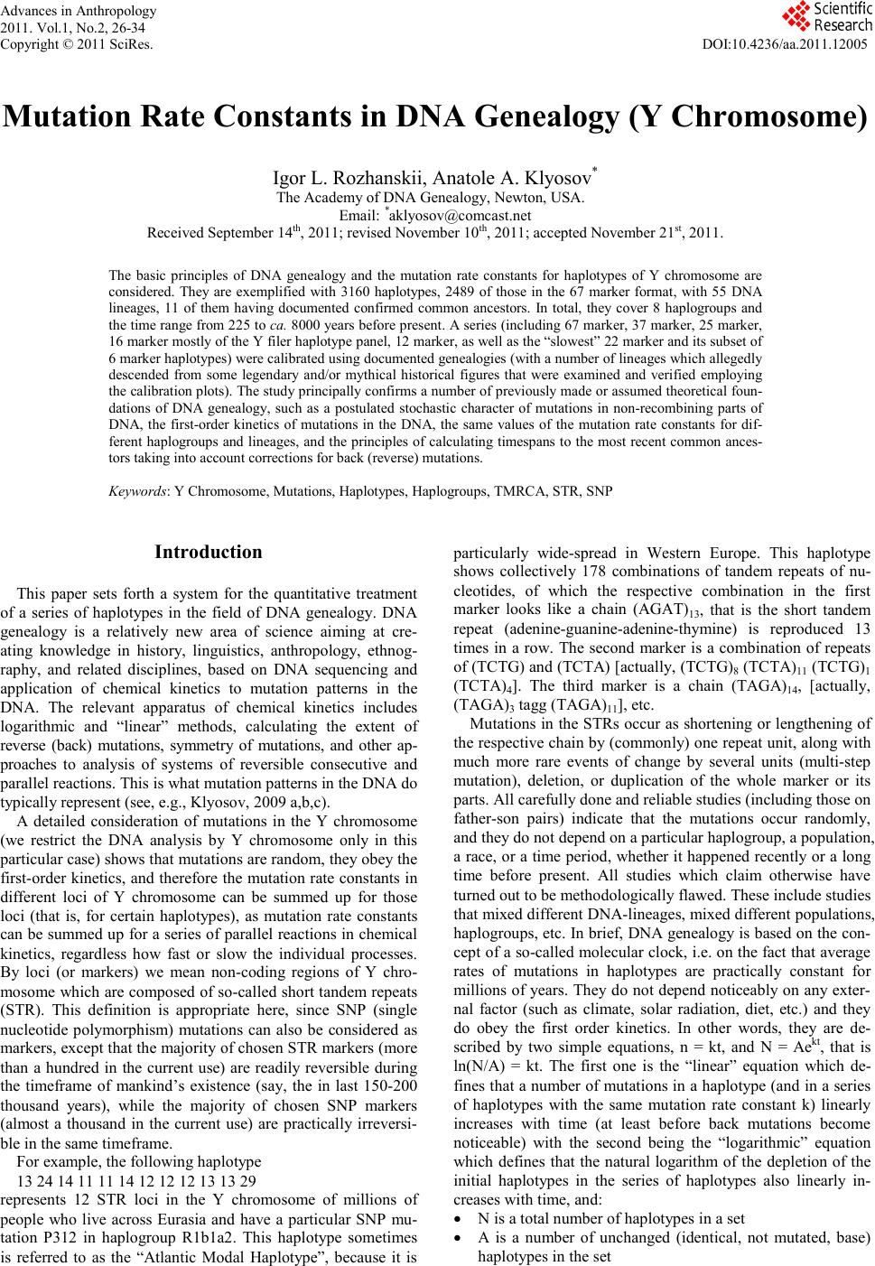
 Advances in Anthropology 2011. Vol.1, No.2, 26-34 Copyright © 2011 SciRes. DOI:10.4236/aa.2011.12005 Mutation Rate Constants in DNA Genealogy (Y Chromosome) Igor L. Rozhanskii, Anatole A. Klyosov* The Academy of DNA Genealogy, Newton, USA. Email: *aklyosov@comcast.net Received September 14th, 2011; revised November 10th, 2011; accepted November 21st, 2011. The basic principles of DNA genealogy and the mutation rate constants for haplotypes of Y chromosome are considered. They are exemplified with 3160 haplotypes, 2489 of those in the 67 marker format, with 55 DNA lineages, 11 of them having documented confirmed common ancestors. In total, they cover 8 haplogroups and the time range from 225 to ca. 8000 years before present. A series (including 67 marker, 37 marker, 25 marker, 16 marker mostly of the Y filer haplotype panel, 12 marker, as well as the “slowest” 22 marker and its subset of 6 marker haplotypes) were calibrated using documented genealogies (with a number of lineages which allegedly descended from some legendary and/or mythical historical figures that were examined and verified employing the calibration plots). The study principally confirms a number of previously made or assumed theoretical foun- dations of DNA genealogy, such as a postulated stochastic character of mutations in non-recombining parts of DNA, the first-order kinetics of mutations in the DNA, the same values of the mutation rate constants for dif- ferent haplogroups and lineages, and the principles of calculating timespans to the most recent common ances- tors taking into account corrections for back (reverse) mutations. Keywords: Y Chromosome, Mutations, Haplotypes, Haplogroups, TMRCA, STR, SNP Introduction This paper sets forth a system for the quantitative treatment of a series of haplotypes in the field of DNA genealogy. DNA genealogy is a relatively new area of science aiming at cre- ating knowledge in history, linguistics, anthropology, ethnog- raphy, and related disciplines, based on DNA sequencing and application of chemical kinetics to mutation patterns in the DNA. The relevant apparatus of chemical kinetics includes logarithmic and “linear” methods, calculating the extent of reverse (back) mutations, symmetry of mutations, and other ap- proaches to analysis of systems of reversible consecutive and parallel reactions. This is what mutation patterns in the DNA do typically represent (see, e.g., Klyosov, 2009 a,b,c). A detailed consideration of mutations in the Y chromosome (we restrict the DNA analysis by Y chromosome only in this particular case) shows that mutations are random, they obey the first-order kinetics, and therefore the mutation rate constants in different loci of Y chromosome can be summed up for those loci (that is, for certain haplotypes), as mutation rate constants can be summed up for a series of parallel reactions in chemical kinetics, regardless how fast or slow the individual processes. By loci (or markers) we mean non-coding regions of Y chro- mosome which are composed of so-called short tandem repeats (STR). This definition is appropriate here, since SNP (single nucleotide polymorphism) mutations can also be considered as markers, except that the majority of chosen STR markers (more than a hundred in the current use) are readily reversible during the timeframe of mankind’s existence (say, the in last 150-200 thousand years), while the majority of chosen SNP markers (almost a thousand in the current use) are practically irreversi- ble in the same timeframe. For example, the following haplotype 13 24 14 11 11 14 12 12 12 13 13 29 represents 12 STR loci in the Y chromosome of millions of people who live across Eurasia and have a particular SNP mu- tation P312 in haplogroup R1b1a2. This haplotype sometimes is referred to as the “Atlantic Modal Haplotype”, because it is particularly wide-spread in Western Europe. This haplotype shows collectively 178 combinations of tandem repeats of nu- cleotides, of which the respective combination in the first marker looks like a chain (AGAT)13, that is the short tandem repeat (adenine-guanine-adenine-thymine) is reproduced 13 times in a row. The second marker is a combination of repeats of (TCTG) and (TCTA) [actually, (TCTG)8 (TCTA)11 (TCTG)1 (TCTA)4]. The third marker is a chain (TAGA)14, [actually, (TAGA)3 tagg (TAGA)11], etc. Mutations in the STRs occur as shortening or lengthening of the respective chain by (commonly) one repeat unit, along with much more rare events of change by several units (multi-step mutation), deletion, or duplication of the whole marker or its parts. All carefully done and reliable studies (including those on father-son pairs) indicate that the mutations occur randomly, and they do not depend on a particular haplogroup, a population, a race, or a time period, whether it happened recently or a long time before present. All studies which claim otherwise have turned out to be methodologically flawed. These include studies that mixed different DNA-lineages, mixed different populations, haplogroups, etc. In brief, DNA genealogy is based on the con- cept of a so-called molecular clock, i.e. on the fact that average rates of mutations in haplotypes are practically constant for millions of years. They do not depend noticeably on any exter- nal factor (such as climate, solar radiation, diet, etc.) and they do obey the first order kinetics. In other words, they are de- scribed by two simple equations, n = kt, and N = Aekt, that is ln(N/A) = kt. The first one is the “linear” equation which de- fines that a number of mutations in a haplotype (and in a series of haplotypes with the same mutation rate constant k) linearly increases with time (at least before back mutations become noticeable) with the second being the “logarithmic” equation which defines that the natural logarithm of the depletion of the initial haplotypes in the series of haplotypes also linearly in- creases with time, and: N is a total number of haplotypes in a set A is a number of unchanged (identical, not mutated, base) haplotypes in the set 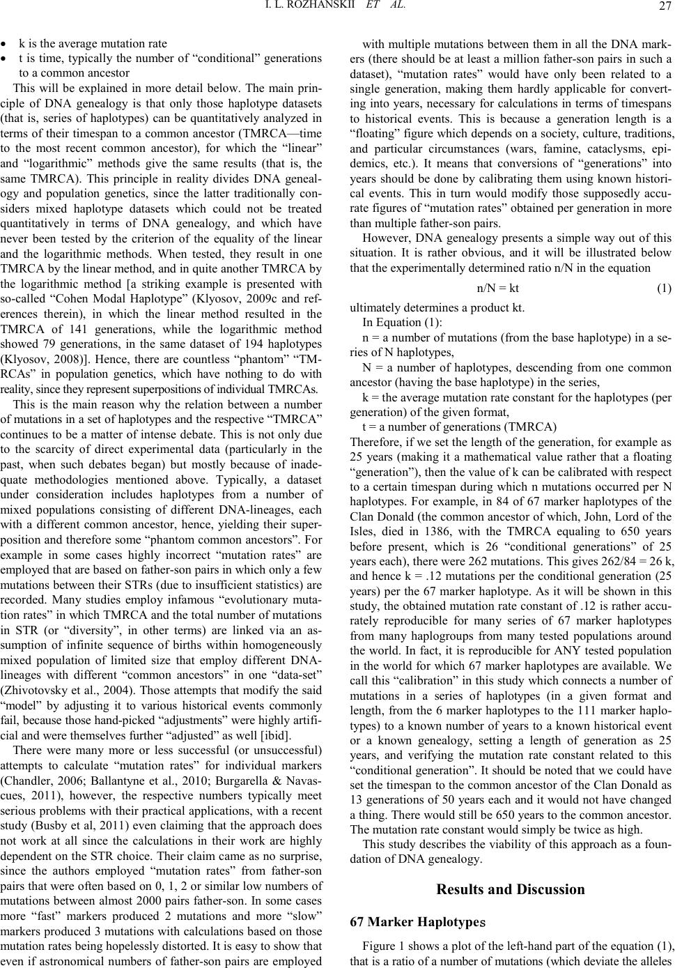 I. L. ROZHANSKII ET AL. 27 k is the average mutation rate t is time, typically the number of “conditional” generations to a common ancestor This will be explained in more detail below. The main prin- ciple of DNA genealogy is that only those haplotype datasets (that is, series of haplotypes) can be quantitatively analyzed in terms of their timespan to a common ancestor (TMRCA—time to the most recent common ancestor), for which the “linear” and “logarithmic” methods give the same results (that is, the same TMRCA). This principle in reality divides DNA geneal- ogy and population genetics, since the latter traditionally con- siders mixed haplotype datasets which could not be treated quantitatively in terms of DNA genealogy, and which have never been tested by the criterion of the equality of the linear and the logarithmic methods. When tested, they result in one TMRCA by the linear method, and in quite another TMRCA by the logarithmic method [a striking example is presented with so-called “Cohen Modal Haplotype” (Klyosov, 2009c and ref- erences therein), in which the linear method resulted in the TMRCA of 141 generations, while the logarithmic method showed 79 generations, in the same dataset of 194 haplotypes (Klyosov, 2008)]. Hence, there are countless “phantom” “TM- RCAs” in population genetics, which have nothing to do with reality, since they represent superpositions of individual TMRCAs. This is the main reason why the relation between a number of mutations in a set of haplotypes and the respective “TMRCA” continues to be a matter of intense debate. This is not only due to the scarcity of direct experimental data (particularly in the past, when such debates began) but mostly because of inade- quate methodologies mentioned above. Typically, a dataset under consideration includes haplotypes from a number of mixed populations consisting of different DNA-lineages, each with a different common ancestor, hence, yielding their super- position and therefore some “phantom common ancestors”. For example in some cases highly incorrect “mutation rates” are employed that are based on father-son pairs in which only a few mutations between their STRs (due to insufficient statistics) are recorded. Many studies employ infamous “evolutionary muta- tion rates” in which TMRCA and the total number of mutations in STR (or “diversity”, in other terms) are linked via an as- sumption of infinite sequence of births within homogeneously mixed population of limited size that employ different DNA- lineages with different “common ancestors” in one “data-set” (Zhivotovsky et al., 2004). Those attempts that modify the said “model” by adjusting it to various historical events commonly fail, because those hand-picked “adjustments” were highly artifi- cial and were themselves further “adjusted” as well [ibid]. There were many more or less successful (or unsuccessful) attempts to calculate “mutation rates” for individual markers (Chandler, 2006; Ballantyne et al., 2010; Burgarella & Navas- cues, 2011), however, the respective numbers typically meet serious problems with their practical applications, with a recent study (Busby et al, 2011) even claiming that the approach does not work at all since the calculations in their work are highly dependent on the STR choice. Their claim came as no surprise, since the authors employed “mutation rates” from father-son pairs that were often based on 0, 1, 2 or similar low numbers of mutations between almost 2000 pairs father-son. In some cases more “fast” markers produced 2 mutations and more “slow” markers produced 3 mutations with calculations based on those mutation rates being hopelessly distorted. It is easy to show that even if astronomical numbers of father-son pairs are employed with multiple mutations between them in all the DNA mark- ers (there should be at least a million father-son pairs in such a dataset), “mutation rates” would have only been related to a single generation, making them hardly applicable for convert- ing into years, necessary for calculations in terms of timespans to historical events. This is because a generation length is a “floating” figure which depends on a society, culture, traditions, and particular circumstances (wars, famine, cataclysms, epi- demics, etc.). It means that conversions of “generations” into years should be done by calibrating them using known histori- cal events. This in turn would modify those supposedly accu- rate figures of “mutation rates” obtained per generation in more than multiple father-son pairs. However, DNA genealogy presents a simple way out of this situation. It is rather obvious, and it will be illustrated below that the experimentally determined ratio n/N in the equation n/N = kt (1) ultimately determines a product kt. In Equation (1): n = a number of mutations (from the base haplotype) in a se- ries of N haplotypes, N = a number of haplotypes, descending from one common ancestor (having the base haplotype) in the series, k = the average mutation rate constant for the haplotypes (per generation) of the given format, t = a number of generations (TMRCA) Therefore, if we set the length of the generation, for example as 25 years (making it a mathematical value rather that a floating “generation”), then the value of k can be calibrated with respect to a certain timespan during which n mutations occurred per N haplotypes. For example, in 84 of 67 marker haplotypes of the Clan Donald (the common ancestor of which, John, Lord of the Isles, died in 1386, with the TMRCA equaling to 650 years before present, which is 26 “conditional generations” of 25 years each), there were 262 mutations. This gives 262/84 = 26 k, and hence k = .12 mutations per the conditional generation (25 years) per the 67 marker haplotype. As it will be shown in this study, the obtained mutation rate constant of .12 is rather accu- rately reproducible for many series of 67 marker haplotypes from many haplogroups from many tested populations around the world. In fact, it is reproducible for ANY tested population in the world for which 67 marker haplotypes are available. We call this “calibration” in this study which connects a number of mutations in a series of haplotypes (in a given format and length, from the 6 marker haplotypes to the 111 marker haplo- types) to a known number of years to a known historical event or a known genealogy, setting a length of generation as 25 years, and verifying the mutation rate constant related to this “conditional generation”. It should be noted that we could have set the timespan to the common ancestor of the Clan Donald as 13 generations of 50 years each and it would not have changed a thing. There would still be 650 years to the common ancestor. The mutation rate constant would simply be twice as high. This study describes the viability of this approach as a foun- dation of DNA genealogy. Results and Discussion 67 Marker Haplotyp es Figure 1 shows a plot of the left-hand part of the equation (1), that is a ratio of a number of mutations (which deviate the alleles 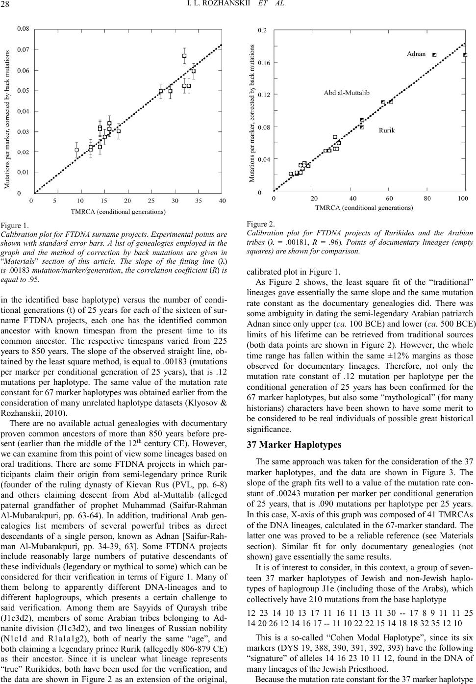 I. L. ROZHANSKII ET AL. 28 Figure 1. Calibration plot for FTDNA surname projects. Experimental points are shown with standard error bars. A list of genealogies employed in the graph and the method of correction by back mutations are given in “Materials” section of this article. The slope of the fitting line (λ) is .00183 mutation/marker/generation, the cor relation co effic ient (R) is equal to .95. in the identified base haplotype) versus the number of condi- tional generations (t) of 25 years for each of the sixteen of sur- name FTDNA projects, each one has the identified common ancestor with known timespan from the present time to its common ancestor. The respective timespans varied from 225 years to 850 years. The slope of the observed straight line, ob- tained by the least square method, is equal to .00183 (mutations per marker per conditional generation of 25 years), that is .12 mutations per haplotype. The same value of the mutation rate constant for 67 marker haplotypes was obtained earlier from the consideration of many unrelated haplotype datasets (Klyosov & Rozhanskii, 2010). There are no available actual genealogies with documentary proven common ancestors of more than 850 years before pre- sent (earlier than the middle of the 12th century CE). However, we can examine from this point of view some lineages based on oral traditions. There are some FTDNA projects in which par- ticipants claim their origin from semi-legendary prince Rurik (founder of the ruling dynasty of Kievan Rus (PVL, pp. 6-8) and others claiming descent from Abd al-Muttalib (alleged paternal grandfather of prophet Muhammad (Saifur-Rahman Al-Mubarakpuri, pp. 63-64). In addition, traditional Arab gen- ealogies list members of several powerful tribes as direct descendants of a single person, known as Adnan [Saifur-Rah- man Al-Mubarakpuri, pp. 34-39, 63]. Some FTDNA projects include reasonably large numbers of putative descendants of these individuals (legendary or mythical to some) which can be considered for their verification in terms of Figure 1. Many of them belong to apparently different DNA-lineages and to different haplogroups, which presents a certain challenge to said verification. Among them are Sayyids of Quraysh tribe (J1c3d2), members of some Arabian tribes belonging to Ad- nanite division (J1c3d2), and two lineages of Russian nobility (N1c1d and R1a1a1g2), both of nearly the same “age”, and both claiming a legendary prince Rurik (allegedly 806-879 CE) as their ancestor. Since it is unclear what lineage represents “true” Rurikides, both have been used for the verification, and the data are shown in Figure 2 as an extension of the original, Figure 2. Calibration plot for FTDNA projects of Rurikides and the Arabian tribes (λ = .00181, R = .96). Points of documentary lineages (empty squares) are shown for comparison. calibrated plot in Figure 1. As Figure 2 shows, the least square fit of the “traditional” lineages gave essentially the same slope and the same mutation rate constant as the documentary genealogies did. There was some ambiguity in dating the semi-legendary Arabian patriarch Adnan since only upper (ca. 100 BCE) and lower (ca. 500 BCE) limits of his lifetime can be retrieved from traditional sources (both data points are shown in Figure 2). However, the whole time range has fallen within the same ±12% margins as those observed for documentary lineages. Therefore, not only the mutation rate constant of .12 mutation per haplotype per the conditional generation of 25 years has been confirmed for the 67 marker haplotypes, but also some “mythological” (for many historians) characters have been shown to have some merit to be considered to be real individuals of possible great historical significance. 37 Marker Haplotypes The same approach was taken for the consideration of the 37 marker haplotypes, and the data are shown in Figure 3. The slope of the graph fits well to a value of the mutation rate con- stant of .00243 mutation per marker per conditional generation of 25 years, that is .090 mutations per haplotype per 25 years. In this case, X-axis of this graph was composed of 41 TMRCAs of the DNA lineages, calculated in the 67-marker standard. The latter one was proved to be a reliable reference (see Materials section). Similar fit for only documentary genealogies (not shown) gave essentially the same results. It is of interest to consider, in this context, a group of seven- teen 37 marker haplotypes of Jewish and non-Jewish haplo- types of haplogroup J1e (including those of the Arabs), which collectively have 210 mutations from the base haplotype 12 23 14 10 13 17 11 16 11 13 11 30 -- 17 8 9 11 11 25 14 20 26 12 14 16 17 -- 11 10 22 22 15 14 18 18 32 35 12 10 This is a so-called “Cohen Modal Haplotype”, since its six markers (DYS 19, 388, 390, 391, 392, 393) have the following “signature” of alleles 14 16 23 10 11 12, found in the DNA of many lineages of the Jewish Priesthood. Because the mutation rate constant for the 37 marker haplotype 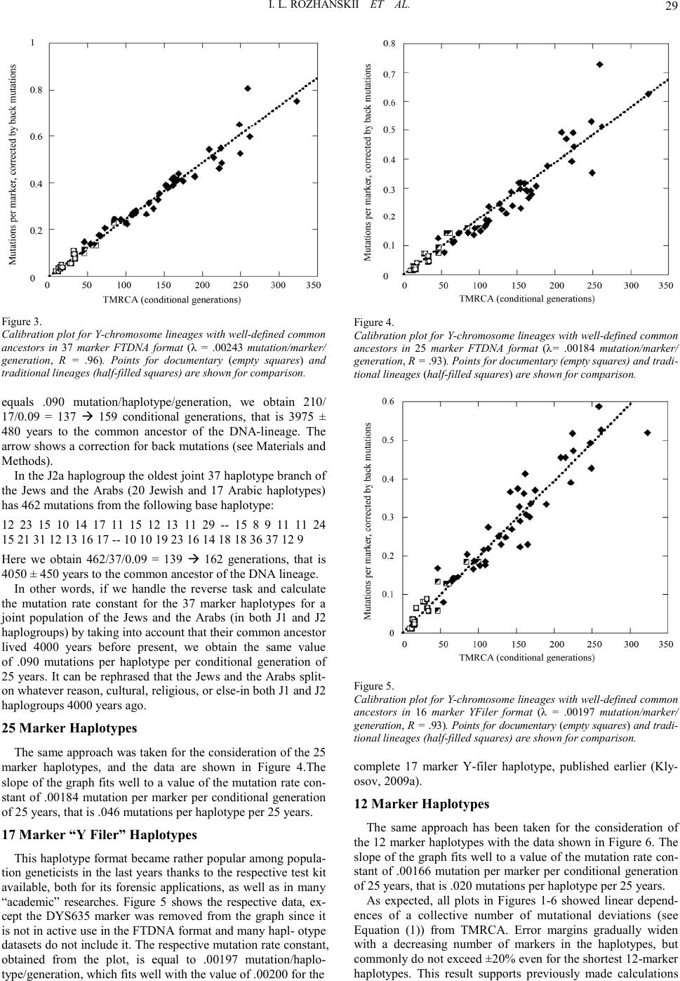 I. L. ROZHANSKII ET AL. 29 Figure 3. Calibration plot for Y-chromosome lineages with well-defined common ancestors in 37 marker FTDNA format (λ = .00243 mutation/marker/ generation, R = .96). Points for documentary (empty squares) and traditional lineages (half-filled squares) are shown for comparison. equals .090 mutation/haplotype/generation, we obtain 210/ 17/0.09 = 137 159 conditional generations, that is 3975 ± 480 years to the common ancestor of the DNA-lineage. The arrow shows a correction for back mutations (see Materials and Methods). In the J2a haplogroup the oldest joint 37 haplotype branch of the Jews and the Arabs (20 Jewish and 17 Arabic haplotypes) has 462 mutations from the following base haplotype: 12 23 15 10 14 17 11 15 12 13 11 29 -- 15 8 9 11 11 24 15 21 31 12 13 16 17 -- 10 10 19 23 16 14 18 18 36 37 12 9 Here we obtain 462/37/0.09 = 139 162 generations, that is 4050 ± 450 years to the common ancestor of the DNA lineage. In other words, if we handle the reverse task and calculate the mutation rate constant for the 37 marker haplotypes for a joint population of the Jews and the Arabs (in both J1 and J2 haplogroups) by taking into account that their common ancestor lived 4000 years before present, we obtain the same value of .090 mutations per haplotype per conditional generation of 25 years. It can be rephrased that the Jews and the Arabs split- on whatever reason, cultural, religious, or else-in both J1 and J2 haplogroups 4000 years ago. 25 Marker Haplotypes The same approach was taken for the consideration of the 25 marker haplotypes, and the data are shown in Figure 4.The slope of the graph fits well to a value of the mutation rate con- stant of .00184 mutation per marker per conditional generation of 25 years, that is .046 mutations per haplotype per 25 years. 17 Marker “Y Filer” Haplotypes This haplotype format became rather popular among popula- tion geneticists in the last years thanks to the respective test kit available, both for its forensic applications, as well as in many “academic” researches. Figure 5 shows the respective data, ex- cept the DYS635 marker was removed from the graph since it is not in active use in the FTDNA format and many hapl- otype datasets do not include it. The respective mutation rate constant, obtained from the plot, is equal to .00197 mutation/haplo- type/generation, which fits well with the value of .00200 for the Figure 4. Calibration plot for Y-chromosome lineages with well-defined common ancestors in 25 marker FTDNA format (λ= .00184 mutation/marker/ generation, R = .93). Points for documentary (empty s qu ar es ) and tradi- tional lineages (hal f-filled squares) are shown for comparison. Figure 5. Calibration plot for Y-chromosome lineages with well-defined common ancestors in 16 marker YFiler format (λ = .00197 mutation/marker/ generation, R = .93). Points for documentary (empty squares) and tradi- tional lineages (half-filled square s) are s hown for comparison. complete 17 marker Y-filer haplotype, published earlier (Kly- osov, 2009a). 12 Marker Haplotypes The same approach has been taken for the consideration of the 12 marker haplotypes with the data shown in Figure 6. The slope of the graph fits well to a value of the mutation rate con- stant of .00166 mutation per marker per conditional generation of 25 years, that is .020 mutations per haplotype per 25 years. As expected, all plots in Figures 1-6 showed linear depend- ences of a collective number of mutational deviations (see Equation (1)) from TMRCA. Error margins gradually widen with a decreasing number of markers in the haplotypes, but commonly do not exceed ±20% even for the shortest 12-marker haplotypes. This result supports previously made calculations 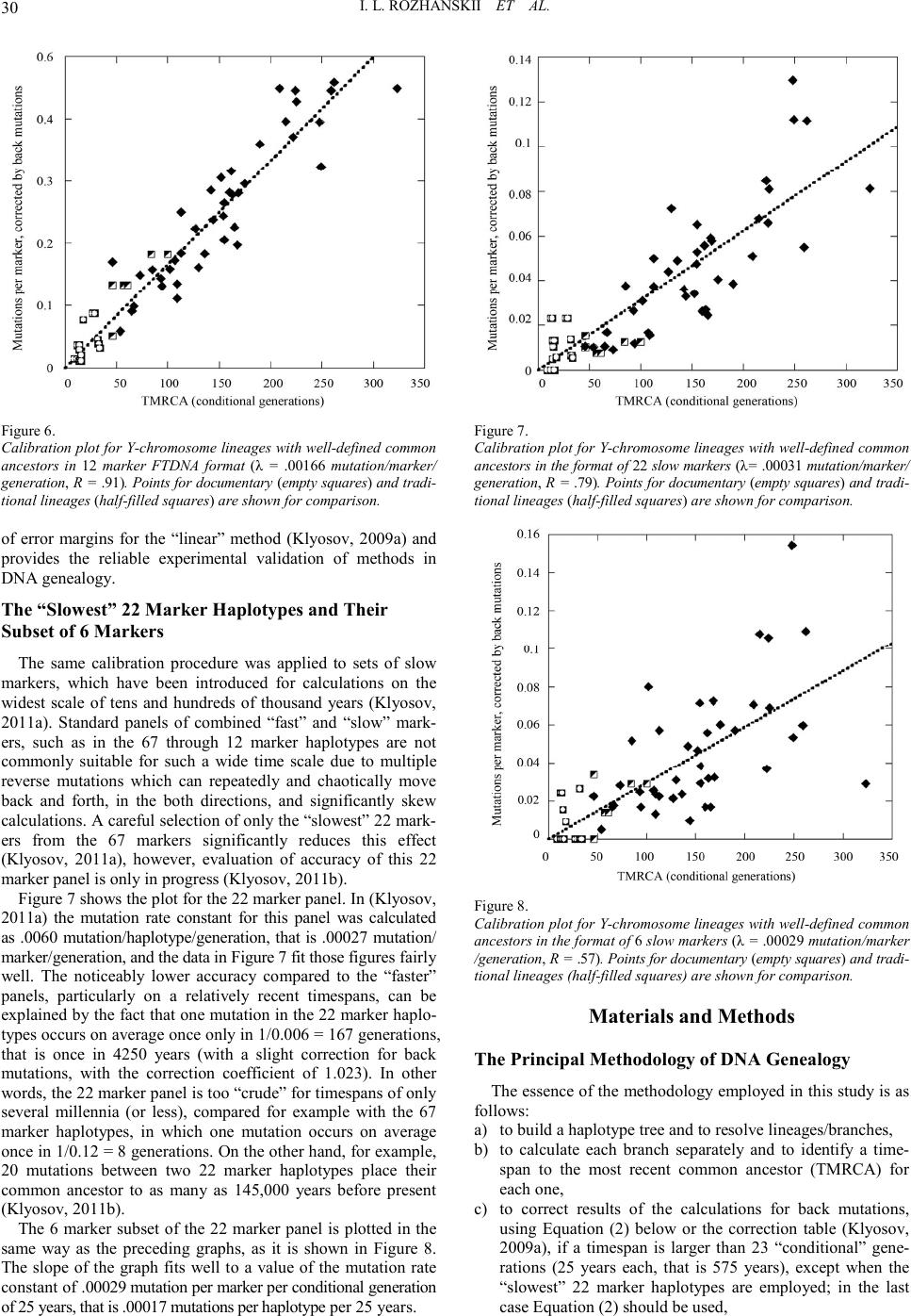 I. L. ROZHANSKII ET AL. 30 Figure 6. Calibration plot for Y-chromosome lineages with well-defined common ancestors in 12 marker FTDNA format (λ = .00166 mutation/marker/ generation, R = .91). Points for documentary (empty squares) and tradi- tional lineages (half-filled squares) are shown for comparison. of error margins for the “linear” method (Klyosov, 2009a) and provides the reliable experimental validation of methods in DNA genealogy. The “Slowest” 22 Marker Haplotypes and Their Subset of 6 Markers The same calibration procedure was applied to sets of slow markers, which have been introduced for calculations on the widest scale of tens and hundreds of thousand years (Klyosov, 2011a). Standard panels of combined “fast” and “slow” mark- ers, such as in the 67 through 12 marker haplotypes are not commonly suitable for such a wide time scale due to multiple reverse mutations which can repeatedly and chaotically move back and forth, in the both directions, and significantly skew calculations. A careful selection of only the “slowest” 22 mark- ers from the 67 markers significantly reduces this effect (Klyosov, 2011a), however, evaluation of accuracy of this 22 marker panel is only in progress (Klyosov, 2011b). Figure 7 shows the plot for the 22 marker panel. In (Klyosov, 2011a) the mutation rate constant for this panel was calculated as .0060 mutation/haplotype/generation, that is .00027 mutation/ marker/generation, and the data in Figure 7 fit those figures fairly well. The noticeably lower accuracy compared to the “faster” panels, particularly on a relatively recent timespans, can be explained by the fact that one mutation in the 22 marker haplo- types occurs on average once only in 1/0.006 = 167 generations, that is once in 4250 years (with a slight correction for back mutations, with the correction coefficient of 1.023). In other words, the 22 marker panel is too “crude” for timespans of only several millennia (or less), compared for example with the 67 marker haplotypes, in which one mutation occurs on average once in 1/0.12 = 8 generations. On the other hand, for example, 20 mutations between two 22 marker haplotypes place their common ancestor to as many as 145,000 years before present (Klyosov, 2011b). The 6 marker subset of the 22 marker panel is plotted in the same way as the preceding graphs, as it is shown in Figure 8. The slope of the graph fits well to a value of the mutation rate constant of .00029 mutation per marker per conditional generation of 25 years, that is .00017 mutations per haplotype per 25 years. Figure 7. Calibration plot for Y-chromosome lineages with well-defined common a nces tors i n the fo rmat of 22 slow markers (λ= .00031 mutation/marker/ generation, R = .79). Points for documentary (empty squares) and tradi- tional lineages (half-filled squares) are shown for comparison. Figure 8. Calibration plot for Y-chromosome lineages with well-defined common ancestors in the format of 6 slow markers (λ = .00029 muta tion /marke r /generation, R = .57). Points for documentary (empty squares) an d tradi - tional lineages (half-filled square s) are s hown for comparison. Materi als and Me tho ds The Principal Methodology of DNA Genealogy The essence of the methodology employed in this study is as follows: a) to build a haplotype tree and to resolve lineages/branches, b) to calculate each branch separately and to identify a time- span to the most recent common ancestor (TMRCA) for each one, c) to correct results of the calculations for back mutations, using Equation (2) below or the correction table (Klyosov, 2009a), if a timespan is larger than 23 “conditional” gene- rations (25 years each, that is 575 years), except when the “slowest” 22 marker haplotypes are employed; in the last case Equation (2) should be used, 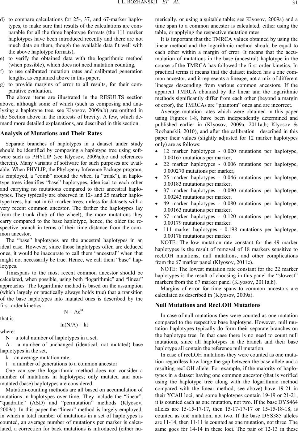 I. L. ROZHANSKII ET AL. 31 d) to compare calculations for 25-, 37, and 67-marker haplo- types, to make sure that results of the calculations are com- parable for all the three haplotype formats (the 111 marker haplotypes have been introduced recently and there are not much data on them, though the available data fit well with the above haplotype formats), e) to verify the obtained data with the logarithmic method (when possible), which does not need mutation counting, f) to use calibrated mutation rates and calibrated generation lengths, as explained above in this paper, g) to provide margins of error to all results, for their com- parative evaluation. The above items are illustrated in the RESULTS section above, although some of which (such as composing and ana- lyzing a haplotype tree, see Klyosov, 2009a,b) are omitted in the Section above in the interests of brevity. A few, which de- mand more detailed explanations, are described in this section. Analysis of Mutations and Their Rates Separate branches of haplotypes in a dataset under study should be identified by composing a haplotype tree using soft- ware such as PHYLIP (see Klyosov, 2009a,b,c and references therein). Many variants of software for such purposes are avail- able. When PHYLIP, the Phylogeny Inference Package program, is employed, a “comb” around the wheel (a “trunk”), in haplo- type trees identifies “base” haplotypes, identical to each other and carrying no mutations compared to their ancestral haplo- types. They typically are observed in 12- and 25 marker haplo- type trees, but not in 67 marker trees, unless for datasets with a very recent common ancestor. The farther the haplotypes lay from the trunk (hub of the wheel), the more mutations they carry compared to the base haplotype, hence, the older the re- spective branch in terms of their time distance from the com- mon ancestor. The “base” haplotypes are the ancestral haplotypes in an ideal case. However, since those haplotypes often are deduced ones, it would be inaccurate to call them “ancestral” when that might not necessarily be true. Hence, we call them “base” hap- lotypes. Timespans to the most recent common ancestor should be calculated, when possible, using both “logarithmic” and “linear” approaches. The logarithmic method is based on the assumption (which largely or practically always holds true) that a transition of the base haplotypes into mutated ones is described by the first-order kinetics: N = Aekt, that is ln(N/A) = kt where: N = a total number of haplotypes in a set, A = a number of unchanged (identical, not mutated) base haplotypes in the set, k = an average mutation rate, t = a number of generations to a common ancestor. One can see the logarithmic method does not consider a number of mutations in haplotypes; only mutated and non- mutated (base) haplotypes are considered. Mutation-counting methods are all based on accumulation of mutations in haplotypes over time. They include the “linear”, “quadratic” (ASD) and “permutation” methods (Klyosov, 2009a). In this paper the “linear” method is largely employed, in which a total number of mutations in a set of haplotypes is counted, an average number of mutations per marker is calcu- lated, a correction for back mutations is introduced (either nu- merically, or using a suitable table; see Klyosov, 2009a) and a time span to a common ancestor is calculated, either using the table, or applying the respective mutation rates. It is important that the TMRCA values obtained by using the linear method and the logarithmic method should be equal to each other within a margin of error. It means that the accu- mulation of mutations in the base (ancestral) haplotype in the course of the TMRCA has followed the first order kinetics. In practical terms it means that the dataset indeed has a one com- mon ancestor, and it represents a lineage, not a mix of different lineages descending from various common ancestors. If the apparent TMRCA obtained by the linear and the logarithmic methods significantly differ from each other (beyond a margin of error), the TMRCAs are “phantom” ones and are incorrect. Average mutation rates which were obtained in this paper using Figures 1-8, have been independently determined and published earlier in (Klyosov, 2009a, 2011a,b; Klyosov & Rozhanskii, 2010), and after the calibration described in this paper their values (slightly adjusted for 12 marker haplotypes only) are as follows: 12 marker haplotypes - 0.020 mutations per haplotype, 0.00167 mutations per marker, 22 marker haplotypes - 0.006 mutations per haplotype, 0.000270 mutations per marker, 25 marker haplotypes - 0.046 mutations per haplotype, 0.00183 mutations per marker, 37 marker haplotypes - 0.090 mutations per haplotype, 0.00243 mutations per marker, 49 marker haplotypes - 0.080 mutations per haplotype, 0.00163 mutations per marker, 67 marker haplotypes - 0.120 mutations per haplotype, 0.00179 mutations per marker. 111 marker haplotypes - 0.198 mutations per haplotype, 0.00178 mutations per marker. NOTE: The low mutation rate constant for the 49 marker haplotypes is the result of removal of 18 markers sensitive to recLOH mutations, null mutations, and other complications from the 67 marker panel (Klyosov, 2011c). NOTE: The lowest mutation rate constant for the 22 marker haplotypes is the result of choosing in this panel the “slowest” markers from the 67 marker panel (Klyosov, 2011a,b). Margins of error for time spans to common ancestors are calculated as described in (Klyosov, 2009a). Null Mutations and RecLOH Mutations In case of null mutations they were counted as one mutation compared to the respective base haplotype. However, null mu- tation haplotypes typically do form their separate branches on the haplotype tree. In that case there is no need to count null mutations, since all haplotypes in the branch and their base haplotype all contain the reference null mutation. In case of recLOH mutations they were counted as one muta- tion regardless how large the gap between the base allele and a resulting recLOH allele. For example, if the majority of haplo- types in a dataset having one common ancestor (that is verified using the haplotype tree along with the logarithmic method compared with the linear method, see above) have 19-21 in their YCAII loci, and some haplotypes contain 19-19 or 21-21, it is counted each as one mutation, not two. If the base DYS464 alleles are 15-15-17-17, then 15-17-17-17 or 15-15-18-18, is counted as one mutation, not two. If the base DYS385 alleles are 11-14, then 11-11 is counted as one mutation, not three. The same goes for 14-14 in these loci. The pair of 12-13 in these 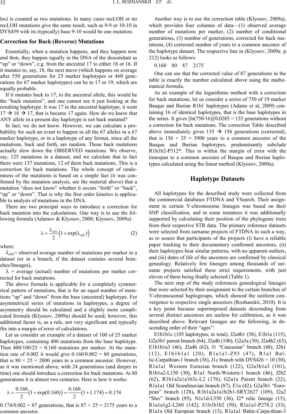 I. L. ROZHANSKII ET AL. 32 loci is counted as two mutations. In many cases recLOH or no recLOH mutations give the same result, such as 9-9 or 10-10 in DYS459 with its (typically) base 9-10 would be one mutation. Correction for Back (Reverse) Mutations Essentially, when a mutation happens, and they happen now and then, they happen equally in the DNA of the descendant as “up” or “down”, e.g. from the ancestral 17 to either 18 or 16. If it mutates to, say, 18, the next move (which happens on average after 550 generations for 25 marker haplotypes or 460 gene- rations for 67 marker haplotypes) can be to 17 or 19, which are equally probable. If it mutates back to 17, to the ancestral allele, this would be the “back mutation”, and one cannot see it just looking at the resulting haplotype. It was 17 in the ancestral haplotype, it went 17 18 17, that is became 17 again. How do we know that ANY allele in a present day haplotype is not back mutated? In fact, we do not know. However, we can calculate a pro- bability for such an event to happen in all the 67 alleles in a 67 marker haplotype, or in a haplotype of any format, since all the mutations, back and forth, are random. Those back mutations actually slow down the OBSERVED mutations. We observe, say, 125 mutations in a dataset, and we calculate that in fact there were 137 mutations, 12 of them back mutations. This is a correction for back mutations. The whole concept of rando- mness of the mutations is based on a simple fact (it was con- firmed by the mutation analysis, see the material above) that a mutation “does not know” whether it occurs “forth” or “back”, “up” or “down”. That is why the first order kinetics is applica- ble to analysis of mutations in the DNA. There are two principal ways to introduce a correction for back mutation into the calculations. One way is to use the fol- lowing formula (Adamov & Klyosov, 2008; Klyosov, 2009a) λ λ1exp(λ) 2 obs obs (2) where: λobs= observed average number of mutations per marker in a dataset (or in a branch, if the dataset contains several bran- ches/lineages), λ = average (actual) number of mutations per marker cor- rected for back mutations. The above formula is applicable for a completely symmet- rical pattern of mutations, that is for an equal number of muta- tions “up” and “down” from the base (ancestral) haplotype. For asymmetrical series of mutations in haplotypes, a degree of asymmetry should be calculated and a slightly more compli- cated formula (Klyosov, 2009a) should be used; however, this additional factor is, as a rule, not very significant and typically fits into a margin of error of calculations. Let us consider an example of a dataset of 100 of 25 marker haplotypes, containing 400 mutations from the base haplotype. Then 400/100/25 = 0.160 mutations per marker. At the muta- tion rate of 0.002 it would give 0.160/0.002 = 80 generations, that is 80 × 25 = 2000 years to a common ancestor. However, as it was mentioned above, with 24 generations (and deeper in time) one should introduce a correction for back mutations. At 80 generations it is almost two centuries. Here is how it works: 0.160 0.160 λ1exp(0.160)1 1.1740.174 22 0.174/0.002 = 87 generations, that is 87 × 25 = 2175 years to a common ancestor. Another way is to use the correction table (Klyosov, 2009a), which provides four columns of data—(1) observed average number of mutations per marker, (2) number of conditional generations, (3) number of generations, corrected for back mu- tations, (4) corrected number of years to a common ancestor of the haplotype dataset. The respective line in (Klyosov, 2009a: p. 212) looks as follows: 0.160 80 87 2175 One can see that the corrected value of 87 generations in the table is exactly the number calculated above using the mathe- matical formula. As an example of the logarithmic method with a correction for back mutations, let us consider a series of 750 of 19 marker Basque and Iberian R1b1 haplotypes (Adams et al, 2009) con- taining 16 of identical haplotypes, that is the base haplotypes in the series. It gives [ln(750/16)]/0.0285 = 135 generations without a correction for back mutations. The correction Table described above immediately gives 135 156 generations (corrected), that is 156 × 25 = 3900 years to a common ancestor of the Basque and Iberian haplotypes, predominantly subclade R1b1b2-P312*. This is within the margin of error with the timespan to a common ancestor of Basque and Iberian haplo- types calculated using the linear method (Klyosov, 2009a). Haplotype Datasets All haplotypes for the described study were collected from the commercial databases FTDNA and YSearch. Their assign- ment to certain Y-chromosome lineages was based on their SNP classification, and in some instances it was additionally supported by calculating their position of the phylogenic trees from their respective STR data. The primary reference datasets were selected from surname projects of FTDNA in such a way, as to assure that participants of the projects (i) have a reliable paper tracking to their documentary confirmed ancestors, (ii) their haplotypes bear similar patterns, with no apparent outliers, and (iii) dates of life of the ancestors are confirmed by classical genealogy. Relatively few lineages among thousands of sur- name projects satisfied these strict requirements, with just eleven of them being finally selected (Table 1). The next step of the study references genealogical lineages that were selected by their assignment to the certain branches of Y-chromosomal haplogroups, which showed the uniform con- vergence to respective single ancestors (Rozhanskii, 2010). It is a key point because superimposed datasets descending from several distinct ancestors are useless for calibration, as it was described above. Relevant lineages are the following, in de- scending order of their “ages”: E1b1b1c (105 haplotypes, in total), J2a4b1 (58), E1b1a (115), G2a3b1 parent branch (64), J2a4b (100), G2a3a (30), J2a4h2 (63), E1b1b1a3 (46), J2a4h (62), J1 “Caucasian” branch (48), J2b1 (12), E1b1b1a1 (20), R1a1a1-Z93 (47), R1a1 Bal- tic-Carpathian-1 branch (38), J1c branch with DYS426 = 10 (30), R1a1a1 Western Eurasian branch (122), G2a3b1a3 (101), R1b1a2-L150 (30), R1a1 North-Western-1 branch (46), J2b2 (62), R1b1a2a1a1b3c-L2 (176), G2a1a Parent branch (22), R1a1a1 Old Scandinavian branch (87), E1a (42), G2a3b1 “Euro- pean” branch (128), R1b1a2a1a1b2b1-SRY2627 (109), I2a2 “Slav” branch (95), N1c1d-L550 (36), I2* relic lineage (15), R1a1a1g2-L260 (142), E1b1b1b2 (50), R1a1a1-P278.2 (33), R1a1a Old European branch (13), R1a1a1 Baltic-Carpa-thian-3  I. L. ROZHANSKII ET AL. 33 Table 1. List of documenta ry g enealogical lineages used for ca librat ion of mutation rates. Links to correspond ing FTDNA projects are given in Appendix. Lineage Haplogroup & subclade Number of participants Ancestor’s life dates Country of origin I Q1b1 17 1720 - after 1775 Germany II R1a1a1g 7 ca. 1663-1713 Germany or France III G2a3b2 20 immigrated 1661 Ireland IV R1a1a1h 22 1614-1652 England V J1 22 b. ca. 1605 England VI R1a1a1 32 b. ca. 1605 England VII A1a 18 b. ca. 1565 England VIII N1c1d 4 ca. 1275-1341 Lithuania IX R1b1a2a1b 11 ca. 1174-1214 Scotland or Belgium X R1a1a1 33 d. 1205 Belgium or England XI R1a1a1h 44 d. 1156 Scotland branch (50), R1a1a1 Northern Eurasian branch (82), R1a1a1 Northern Carpathian branch (33), Q1a3-L213 “Scandinavian” branch (12), R1b1a2a1a1b4b-M222 (287), R1a1a1-L342.2 Ash- kenazi branch (94), J1c3 Ashkenazi branch (45). In total, the reference datasets contained 3160 haplotypes, with 2489 of them being listed in 67-marker format. The calibration was carried out by the linear regression analysis of ancestors’ life dates, expressed in conditional gen- erations (of 25 years each) before present and rounded to inte- gers vs. average mutational distances from presumed ancestral haplotypes in their descendants. The correction for back muta- tions was introduced in Figures 1-8 according to formula (2) above. The λ value in Equation (2) has the same meaning as the variance in the average square distance (ASD) method (Gold- stein et al, 1995a,b). Both the ASD and the “linear” (as in of Equation (1)) methods are equivalent with respect to their mathematical background with the ASD being rather sensitive to multi-step mutations and the presence of small fractions of irrelevant haplotypes in the dataset. In practice it leads, in some cases, to deviations from actual variance values and to the broadening of margins of errors. In this study we preferred to deal with a more stable and reproducible “linear” approach. Throughout this work, average distances were calculated for entire haplotypes, rather than for individual markers. Although any arbitrarily chosen set of markers can be calibrated by this way, the present study is focused on the standard ones which are the most represented in commercial databases and academic publications. These are the FTDNA “standard panels”, consist- ing of 12, 25, 37 and 67 markers, along with 17-marker Y Filer set, which is a default standard in YHRD database and increas- ingly popular in academic studies. In fact, the latter one is stud- ied in this work in its shortened 16-marker version because DYS635 marker is absent in standard FTDNA panels, and there are not enough data for the respective alleles of DYS635 in reference datasets. In addition, calibration was made for the set of 22 markers with intrinsically slow mutation rates, which ap- peared to be a valuable tool for deep ancestry reconstructions (Klyosov, 2011a). These slow 22 markers are listed below in the FTDNA conventional order: DYS426, DYS388, DYS392, DYS455, DYS454, DYS438, DYS531, DYS578, DYS395S1a, DYS395S1b, DYS590, DYS641, DYS472, DYS425, DYS594, DYS436, DYS490, DYS450, DYS617, DYS568, DYS640, DYS492. Since the great majority of these markers belongs to the so-called 4th FTDNA panel, which is not used in many short haplotypes that is typical for “academic studies”, the 6 marker subset was also examined. It consists of 6 underlined markers in the list above. Prior to the linear regression analysis, self-consistency of mutational distances for different sets of markers has been eva- luated from correlation coefficients and calculated for pairs of λ values in 60 lineages (Table 2). Calculated correlation coeffi- cients were as high as .95 - .98 for standard panels showing some increase for pairs with higher number of markers. Corre- lation coefficients for sets of slow markers typically are within the range of .70 - .85, which is consistent with higher scattering of experimental points in “slow” marker haplotypes. Table 2. Correlation coefficients between average mutational distances, cal- culated for different standards. The first column shows a number of markers in the haplotype. # 12 16 25 37 67 6 22 12 1 16 .9801 25 .961.9691 37 .942.965.978 1 67 .949.962.961 .983 1 6 (slow).723.743.710 .698 .695 1 22 (slow).794 .818 .792 .807 .850 .7521  I. L. ROZHANSKII ET AL. 34 References Adamov, D., & Klyosov, A. A. (2008). Theoretical and practical evaluations of back mutations in haplotypes of Y chromosome. Pro- ceedings of the Ru ssian Academy of DNA Gen ealogy, 1, 631-645. Adams, S. M., Bosch, E., Balaresque, P. L., Ballereau, S. J., Lee, A. C., Arroyo, E. et al. (2008). The genetic legacy of religious diversity and intolerance: Paternal lineages of Christians, Jews, and Muslims in the Iberian Peninsula. The American Journal of Human Genetics, 83, 725-736. doi:10 .1016 /j. ajh g.20 08.11 .0 07 Al-Mubarakpuri, S.-R. (2002). The Sealed Nectar (Ar-Raheeq Al- Makhtum). Houston, TX: Dar-us-Salam Publications, 440. Ballantyne, K. N., Goedbloed, M., Fang, R., Schaap, O., Lao, O., Woll- stein, A. et al. (2010). Mutability of Y-chromosomal microsatellites: Rates, characteristic, molecular bases, and forensic implications. The Americ a n Jo urna l of Human Gen et ics, 7, 341-353. doi:10 .1 016/j .aj h g.2010 .08.0 06 Burgarella, С., & Navascues, М. (2011). Mutation rate estimates for 110 Y chromosome STRs combining population and father-son pair data. European Journal of Human Genetics, 19, 70-75. doi:10 .1 038/ ejhg. 2010. 154 Busby, G. B. J., Brisighelli, F., Sánchez-Diz, P., Ramos-Luis, E., Mar- tinez-Cadenas, C., Thomas, M. J. et al. (2011). The peopling of Europe and the cautionary tale of Y chromosome lineage R-M269. Proceeding of the Royal Society B, published online before print August 24. Chandler, J. F. (2006). Estimating per-locus mutation rates. Journal of Genetic Genealogy, 2, 27-33. Goldstein, D. B., Linares, A. R., Cavalli-Sforza, L. L., & Feldman, M. W. (1995). Genetic absolute dating based on microsatellites and the origin of modern humans. Proceeding of the National Academy of Sciences of US, 92, 6723- 6727. Goldstein, D. B., Linares, A. R., Cavalli-Sforza, L. L., & Feldman, M. W. (1995). An evaluation of genetic distances for use with microsa- tellite loci. Genetics , 139, 463-471. Klyosov, A. A. (2008). Origin of the Jews via DNA genealogy. Pro- ceedings of the Russian Academy of DNA Genealogy, 1, 54-232. Klyosov, A. A. (2009a). DNA Genealogy, mutation rates, and some historical evidences written in Y-chromosome. I. Basic principles and the method. Journal of Genetic Genealogy, 5, 186-216. Klyosov, A. A. (2009b). DNA Genealogy, mutation rates, and some historical evidences written in Y-chromosome. II. Walking the map. Journal of Genetic Genealo gy, 5, 217-256. Klyosov, A. A. (2009c). A comment on the paper: Extended Y chromo- some haplotypes resolve multiple and unique lineages of the Jewish priesthood. Human Genetics, 126, 719-72 4. doi:10 .1007 / s00439 -009 -0739-1 Klyosov, A. A. (2011a). The slowest 22 marker haplotype panel (out of the 67 marker panel) and their mutation rate constants employed for calculations timespans to the most ancient common ancestors. Pro- ceedings of the Ru ssian Acad emy of DNA Geneal og, 4, 1240-1257. Klyosov, A. A. (2011b). DNA genealogy of major haplogroups of Y chromosome (Part 1). Proceedings of the Russian Academy of DNA Gene al ogy, 4, 1258-1283. Klyosov, A. A. (2011c). Haplotypes of R1b1a2-P312 and related sub- clades: Origin and “ages” of most recent common ancestors. Pro- ceedings of the Russian Academy of DNA Genealogy, 4, 1127-1195. Klyosov, A. A., & Rozhanskii, I. L. (2010). Revision оf the average mutation rate constant for 67-marker haplotypes—From 0.145 to 0.120 mutations per haplotype per generation (in Russian). Proceed- ings of the Russi an Aca demy of DNA G enealo gy, 3, 2039-2058. PVL: Povest’ Vremennykh Let (1953). The Russian Primary Chronicle, Laurentian Text. Translated and Edited by S. H. Cross & O. P. Sher- bowitz-Wetzor. Cambridge, MA: The Mediaeval Academy of America, 313. Rozhanskii, I. (2010). Evaluation оf the сonvergence оf sets in STR phylogeny and analysis оf the haplogroup R1a1 tree. Proceedings of the Russian Academy of DNA Genealogy, 3, 1316-1324. Zhivotovsky, L. A., Underhill, P. A., Cinnioglu, C., Kayser, M., Morar, B., Kivisild, T. et al. (2004). The effective mutation rate at Y chro- mosome short tandem repeats, with application to human population divergence time. The American Journal of Human Genetics, 74, 50- 61. doi:1 0 .1086/380 911 Appendix The following DNA projects have been selected as primary sources for calibration: http://www.familytreedna.com/public/shockey-schacke/default.aspx http://www.familytreedna.com/public/venter/default.aspx http://www.familytreedna.com/group-join.aspx?Group=Athey http://www.familytreedna.com/public/tucker/default.aspx http://www.familytreedna.com/group-join.aspx?Group=Davenport http://www.familytreedna.com/group-join.aspx?Group=Carpenter http://www.familytreedna.com/group-join.aspx?Group=Bass http://www.familytreedna.com/group-join.aspx?Group=Russian_Nobility http://www.familytreedna.com/group-join.aspx?Group=Dugliss http://www.familytreedna.com/group-join.aspx?Group=Pendergraft http://www.familytreedna.com/group-join.aspx?Group=MacDonald http://www.familytreedna.com/public/sharifs/default.aspx?section=results http://www.familytreedna.com/group-join.aspx?Group=Arab_Tribes Reference data for the second step have been selected according to SNP assignment from YSearch database (http://www.ysearch.org) and public projects of FTDNA (http://www.familytreedna.com)
|