Advances in Pure Mathematics, 2011, 1, 345-350
doi:10.4236/apm.2011.16062 Published Online November 2011 (http://www.SciRP.org/journal/apm)
Application of Adomian’s Decomposition Method for
the Analytical Solution of Space Fractional
Diffusion Equation
Mehdi Safari1, Mohammad Danesh2
1Department of Mechanical Engineering, Islamic Azad University, Aligoodarz Branch, Aligoodarz, Iran
2Department of Mechanical Engineering, Isfahan University of Technology, Isfahan, Iran
Received July 1, 2011; revised September 26, 2011; accepted October 5, 2011
Abstract
Spatially fractional order diffusion equations are generalizations of classical diffusion equations which are
increasingly used in modeling practical super diffusive problems in fluid flow, finance and others areas of
application. This paper presents the analytical solutions of the space fractional diffusion equations by
Adomian’s decomposition method (ADM). By using initial conditions, the explicit solutions of the equations
have been presented in the closed form. Two examples, the first one is one-dimensional and the second one
is two-dimensional fractional diffusion equation, are presented to show the application of the present tech-
niques. The present method performs extremely well in terms of efficiency and simplicity.
Keywords: Adomian’s Decomposition Method, Fractional Derivative, Fractional Diffusion Equation
1. Introduction
Fractional diffusion equations are used to model prob-
lems in Physics [1-3], Finance [4-7], and Hydrology [8-
12]. Fractional space derivatives may be used to formu-
late anomalous dispersion models, where a particle
plume spreads at a rate that is different than the classical
Brownian motion model. When a fractional derivative of
order 1 < α < 2 replaces the second derivative in a diffu-
sion or dispersion model, it leads to a super diffusive
flow model. Nowadays, fractional diffusion equation
plays important roles in modeling anomalous diffusion
and subdiffusion systems, description of fractional ran-
dom walk, unification of diffusion and wave propagation
phenomenon, see, e.g. the reviews in [1-16], and refer-
ences therein. Consider a one-dimensional fractional
diffusion equation considered in [17]
 


,,
,
uxt uxt
dx qxt
tx




, (1)
on a finite domain
L
R
x
xx with 12

. We
assume that the diffusion coefficient (or diffusivity) d(x)
> 0. We also assume an initial condition u(x, t = 0) = s(x)
for
L
R
x
xx
L
ux
and Dirichlet boundary conditions of
the form and

,t0


,
R
t

R
b tux. Equation
(1) uses a Riemann fractio nal derivative of or der

.
Consider a two-dimensional fractional diffusion equa-
tion considered in [18]







,,,, ,,xy
xx

,,
,,
uxytuxytu t
dxy exy
t
qxyt

 



,
(2)
on a finite rectangular domain
L
H
x
xx and
L
R
yyy

, with fractional orders 1 < 2

 and
1 < 2


, where the diffusion coefficients d(x, y) > 0
and e(x, y) > 0. The ‘forcing’ function q(x, y, t) can be
used to represen t sources and sinks. We will assume that
this fractional diffusion equation has a unique and suffi-
ciently smooth solution under the following initial and
boundary conditio ns. Assume the initial condition u(x, y,
t = 0) = f(x, y) for
L
H
x
xx

 and
L
R, and
Dirichlet boundary condition u(x, y, t) = B(x, y, t) on the
boundary (perimeter) of the rectangular region
yyy
L
H
x
xx

,
L
R
yyy

, with the additional restric-
tion that




,t,,yt ,Bxy 0
LL
Bx

. In physical appli-
cations, this means that the left/lower bou ndary is set far
away enough from an evolving plume that no significant
concentrations reach that boundary. The classical disper-
sion equation in two-dimensions is given by 2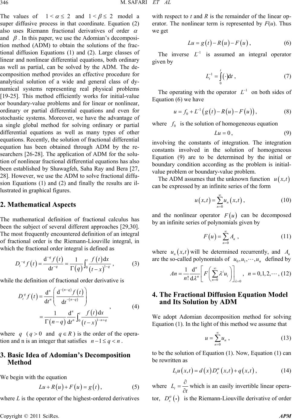



.

M. SAFARI ET AL 346
The values of 1 < 2

 and 1 < 2

 model a
super diffusive process in that coordinate. Equation (2)
also uses Riemann fractional derivatives of order

and

. In this paper, we use the Adomian’s decomposi-
tion method (ADM) to obtain the solutions of the frac-
tional diffusion Equations (1) and (2). Large classes of
linear and nonlinear differential equations, both ordinary
as well as partial, can be solved by the ADM. The de-
composition method provides an effective procedure for
analytical solution of a wide and general class of dy-
namical systems representing real physical problems
[19-25]. This method efficiently works for initial-value
or boundary-value problems and for linear or nonlinear,
ordinary or partial differential equations and even for
stochastic systems. Moreover, we have the advantage of
a single global method for solving ordinary or partial
differential equations as well as many types of other
equations. Recently, the so lution of fractional differential
equation has been obtained through ADM by the re-
searchers [26-28]. The application of ADM for the solu-
tion of nonlinear fractional differential equations has also
been established by Shawagfeh, Saha Ray and Bera [27,
28]. However, we use the ADM to solve fractional diffu-
sion Equations (1) and (2) and finally the results are il-
lustrated in graphi cal fi g ures .
2. Mathematical Aspects
The mathematical definition of fractional calculus has
been the subject of several different approaches [29,30].
The most frequently enco untered defin ition of an integral
of fractional order is the Riemann-Liouville integral, in
which the fractional order integral is defined as
 



1
0
d
1t
q
qq
d
d
q
t
f
tftx
Dft qtx




t


, (3)
while the definition of fractional order derivative is







1
0
d
d
dd
d
1d
d
nq
n
q
tnnq
nt
nn
ft
Dfttt
q
f
tx
nq ttx




 


 

, (4)
where ( and q) is the order of the opera-
tion and n is an integ er that satisfies .
q0qR1nq n
3. Basic Idea of Adomian’s Decomposition
Method
We begin with the equati o n



LuR uFugt 

, (5)
where L is the operator of the highest-ordered derivatives
with respect to t and R is the remainder of the linear op-
erator. The nonlinear term is represented by F(u). Thus
we get


Lug tR uFu 

, (6)
The inverse 1 L

is assumed an integral operator
given by

1
0
d
t
t
L
t



, (7)
The operating with the operator on both sides of
Equation (6) we have
1
L




1
0
uf LgtRuFu

 , (8)
where 0
f
is the solution of homogeneous equation
0Lu , (9)
involving the constants of integration. The integration
constants involved in the solution of homogeneous
Equation (9) are to be determined by the initial or
boundary condition according as the problem is initial-
value problem or boundary-value problem.
The ADM assumes that the unknown function


,uxt
can be expressed by an infinite series of the form
 
0
,
n
n
uxtu xt


,
, (10)
and the nonlinear operator

F
u can be decomposed
by an infinite series of polynomials given by

0n n
F
u


A, (11)
where


,
n
uxtwill be determined recurrently, and n
A
are the so-called polynomials of defined by
01
,,,
n
uu u
00
1d , 0,1,2,
!d
n
i
i
n
n
AnF un
n








 


, (12)
4. The Fractional Diffusion Equation Model
and Its Solution by ADM
We adopt Adomian decomposition method for solving
Equation (1). In the light of this method we assume that
0n n
uu




, (13)
to be the solutio n of Equation (1 ). Now, Equation (1) can
be rewritten as




,,
tx
Luxtdx Dxtqxt



,, (14)
where t
Lt



which is an easily invertible linear opera-
tor,


x
D

 is the Riemann-Liouville derivative of order

M. SAFARI ET AL347

.Therefore, by Adomian decomposition method, we
can write,
  
11
0
,,0 ,
txnt
n
uxtuxLdxDuL qxt

 



 




,
(15)
Each term of series (13) is given by Adomian decom-
position method recurrence relation
0,uf (16)


1
1,0 nt xn
uLdxDun
 
,
, (17)
where
  
1
,0, .
t
f
uxL qxt


It is worth noting that once the zeroth component 0
is defined, then the remaining components n can
be completely determined; each term is computed by
using the previous term. As a result, the components
01 are identified and the series solutions thus en-
tirely determined. However, in many cases the exact so-
lution in a closed form may be obtained.
u
1,un
,,uu
Similarly, for Equation (2) using Adomian decompo-
sition method, we can obtain
 
  
1
0
11
0
,, ,,0,
,,,,
txn
n
tynt
n
uxytuxyL dxyDu
LexyD u Lqxyt

























,
(18)
The Adomian decomposition method recurrence
scheme is
0,uf (19)




11
1,,
0,
ntxntyn
uL dxyDuLexyDu
n
 

 (20)
where


 
,,0,, .
t
1
f
uxyL qxyt

5. Numerical Illustration
5.1. Example 1
Let us consider a one-dimensional fractional diffusion
equation for the Equation (1), as taken in [17]
 


1.8
1.8
,,
,
uxt uxt
dx qxt
tx




, (21)
on a finite domain 0 < x < 1, with the diffusion coeffi-
cient
 
2.8 2.8
2.26 0.183634dx xx , (22)
the source/sink function




3
,1e
t
qxtx x

 , (23)
the initial condition


3
,0, for 01ux xx

, (24)
and the boundary conditions




0,0, 1,e, for 0
t
ut utt


, (25)
Implementation of Adomian’s Decomposition Method
Equation (21) can be rewritten in operator form as




1.8
,,
tx
LuxtdxDux tqxt

,, (26)
where t
Lt



symbolizes the easily invertible linear
differential operator,


1.8
x
D

is the Riemann-Liouville
derivative of order 1.8. I f the i nvertible oper a tor

1
0
d
t
t
L
t



is applied to Equation (26), then






111.8
,,
tttx
LLuxtLdxD uxtqxt

,
, (27)
is obtained. By this








11.8
,,0 ,,
tx
uxtuxLdxD uxtqxt

 , (28)
is found. Here the main point is that the solution of the
decomposition method is in the form of
 
0
,
n
n
uxtu xt


,, (29)
Substituting from Equation (29) into Equation (28),
we find
 
  
0
11.8
0
,,0
,,
n
n
txn
n
uxt ux
LdxDuxtqxt















, (30)
is found. Thus according to Equation (7) approximate
solution can be obtained as follows:


3
0,uxt x, (31)



344 34
1,1.000001369 e,
t
uxtxxxtxx

 (32)
 


1.8
21
0
,,
t
x
uxtdxDuxt qxtt
,d, (33)
The approximate solution of the one-dimensional frac-
tional diffusion equation is obtained as




012
,,,uxtuxt uxt uxt

,
, (34)
In Figure 1 we can see the 3-D result of approximate
solution of the one-dimensional fractional diffusion
equation by ADM.

M. SAFARI ET AL 348
Figure 1. For the one-dimensional fractional diffusion
equation with the initial condition (24) of Equation (21),
ADM result for u(x, t).
5.2. Example 2
Let us consider a two-dimensional fractional diffusion
equation for the Equation (2), considered in [18].




  
1.8
1.8
1.6
1.6
,, ,,
,
,,
,,,,
uxyt uxyt
dxy
tx
uxyt
exy qxyt
y






(35)
on a finite rectangular domain 0 < x < 1, 0 < y < 1, for 0
< t < Tend with the diffusion coefficients
 
2.8
,2.2dxyx y 6

, (36)
and
 
2.6
,2 4.6exyxy, (37)
and the forcing function
 
33.6
,,12 e
t
qxytxyxy

 , (38)
with the initial condition

33.6
,,0uxy xy, (39)
and Dirichlet bound ary conditio ns on the re ctangle in th e
form and
, for all .
 
3
,0,0,,0, ,1,e,
t
uxtuytux tx

 

3.6
,e t t y

0t1,uy
Implementation of Adomian’s Decomposition Method
Now, Equation (35) can be rewritten in operator form as







1.8
1.6
,, ,,,
,,,,,,,
tx
y
LuxytdxyDxy t
exyt Du xytq xyt



(40)
where t
Lt



symbolizes the easily invertible linear
differential operator,


1.8
x
D

and and are the
Riemann–Liouville derivatives of order 1.8 and 1.6, re-
spectively.

1.6
y
D
If the invertible operator is applied to

1
0
d
t
t
L

t
Equation (40) , then





 

111.8
1.6
,,, ,,
,,,,,,,
ttt x
y
LLuxytLdxyD uxyt
exyt Du xytq xyt



(41)
is obtained. By this



 

11.8
1.6
(,,) ,,0,,,
,,,,,,,
tx
y
uxytuxyLdxyD uxyt
exyt Du xytqxyt





(42)
is found. Here the main point is that the solution of the
decomposition method is in the form of
 
0
,, ,,
n
n
uxytu xyt


, (43)
Substituting from Equation (43) into Equation (42),
we find
 

 
0
1 1.8
0
1.6
0
,, ,,0
,,,
,,,,,,,
n
n
txn
n
yn
n
uxyt uxy
LdxyD uxyt
exytDuxytqxyt


















(44)
is found.
Thus according to Equation (7) approximate solution
can be obtained as follows:


33.6
0,, ,uxyt xy (45)

18 23 23
344
55
1
18 23
34
55
,,2 2
e2e,
tt
uxytxyxyxy t
xy xy

 

5
(46)
 

 

1.8
21
0
1.6 1
,,,,,
,,,,,,d,
t
x
y
ux ytdx yDux yt
exyt Duxytqxytt


(47)
The approximate solution of the two-dimensional frac-
tional diffusion equation is obtained as




012
,,,uxtuxt uxtuxt

,
In Figure 2 we can see the 3-D result of approximate
, (48)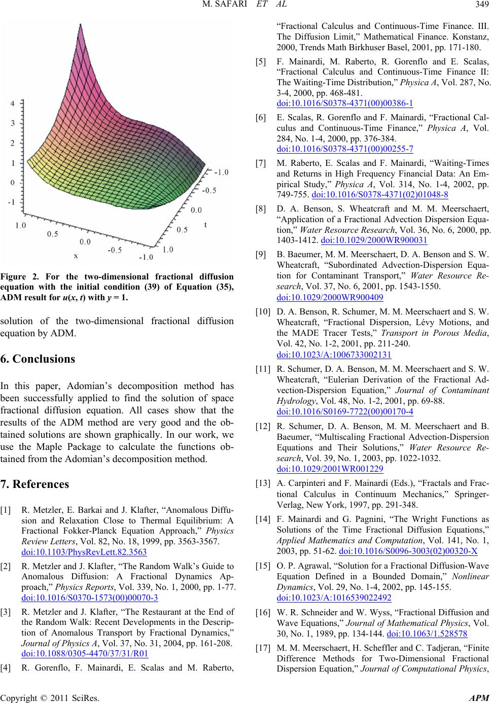

M. SAFARI ET AL349
Figure 2. For the two-dimensional fractional diffusion
lution of the two-dimensional fractional diff
. Conclusions
this paper, Adomian’s decomposition method
. References
] R. Metzler, E. Barkai and J. Klafter, “Anomalous Diffu-
equation with the initial condition (39) of Equation (35),
ADM result for u(x, t) with y = 1.
sousion
equation by ADM.
6
In has
been successfully applied to find the solution of space
fractional diffusion equation. All cases show that the
results of the ADM method are very good and the ob-
tained solutions are shown graphically. In our work, we
use the Maple Package to calculate the functions ob-
tained from the Adomian’s decomposition method.
7
[1 sion and Relaxation Close to Thermal Equilibrium: A
Fractional Fokker-Planck Equation Approach,” Physics
Review Letters, Vol. 82, No. 18, 1999, pp. 3563-3567.
doi:10.1103/PhysRevLett.82.3563
[2] R. Metzler and J. Klafter, “The Random Walk’s Guide to
Anomalous Diffusion: A Fractional Dynamics Ap-
proach,” Physics Reports, Vol. 339, No. 1, 2000, pp. 1-77.
doi:10.1016/S0370-1573(00)00070-3
[3] R. Metzler and J. Klafter, “The Restaurant at the End of
the Random Walk: Recent Developments in the Descrip-
tion of Anomalous Transport by Fractional Dynamics,”
Journal of Physics A, Vol. 37, No. 31, 2004, pp. 161-208.
doi:10.1088/0305-4470/37/31/R01
[4] R. Gorenflo, F. Mainardi, E. Scalas and M. Raberto,
,
00)00386-1
“Fractional Calculus and Continuous-Time Finance. III.
The Diffusion Limit,” Mathematical Finance. Konstanz,
2000, Trends Math Birkhuser Basel, 2001, pp. 171-180.
[5] F. Mainardi, M. Raberto, R. Gorenflo and E. Scalas
“Fractional Calculus and Continuous-Time Finance II:
The Waiting-Time Distribution,” Physica A, Vol. 287, No.
3-4, 2000, pp. 468-481.
doi:10.1016/S0378-4371(
i, “Fractional Cal-
-7
[6] E. Scalas, R. Gorenflo and F. Mainard
culus and Continuous-Time Finance,” Physica A, Vol.
284, No. 1-4, 2000, pp. 376-384.
doi:10.1016/S0378-4371(00)00255
i, “Waiting-Times [7] M. Raberto, E. Scalas and F. Mainard
and Returns in High Frequency Financial Data: An Em-
pirical Study,” Physica A, Vol. 314, No. 1-4, 2002, pp.
749-755. doi:10.1016/S0378-4371(02)01048-8
[8] D. A. Benson, S. Wheatcraft and M. M. Meerschaert,
“Application of a Fractional Advection Dispersion Equa-
tion,” Water Resource Research, Vol. 36, No. 6, 2000, pp.
1403-1412. doi:10.1029/2000WR900031
[9] B. Baeumer, M. M. Meerschaert, D. A. Benson and S. W.
Wheatcraft, “Subordinated Advection-Dispersion Equa-
tion for Contaminant Transport,” Water Resource Re-
search, Vol. 37, No. 6, 2001, pp. 1543-1550.
doi:10.1029/2000WR900409
[10] D. A. Benson, R. Schumer, M. M. Meerschaert and S. W.
Wheatcraft, “Fractional Dispersion, Lévy Motions, and
the MADE Tracer Tests,” Transport in Porous Media,
Vol. 42, No. 1-2, 2001, pp. 211-240.
doi:10.1023/A:1006733002131
[11] R. Schumer, D. A. Benson, M. M. Meerschaert and S. W.
Wheatcraft, “Eulerian Derivation of the Fractional Ad-
vection-Dispersion Equation,” Journal of Contaminant
Hydrology, Vol. 48, No. 1-2, 2001, pp. 69-88.
doi:10.1016/S0169-7722(00)00170-4
[12] R. Schumer, D. A. Benson, M. M. Meerschaert and B.
Baeumer, “Multiscaling Fractional Advection-Dispersion
Equations and Their Solutions,” Water Resource Re-
search, Vol. 39, No. 1, 2003, pp. 1022-1032.
doi:10.1029/2001WR001229
[13] A. Carpinteri and F. Mainardi (Eds.), “Fractals and Frac-
ight Functions as
tional Calculus in Continuum Mechanics,” Springer-
Verlag, New York, 1997, pp. 291-348.
[14] F. Mainardi and G. Pagnini, “The Wr
Solutions of the Time Fractional Diffusion Equations,”
Applied Mathematics and Computation, Vol. 141, No. 1,
2003, pp. 51-62. doi:10.1016/S0096-3003(02)00320-X
[15] O. P. Agrawal, “Solution for a Fractional Diffusion-Wave
Equation Defined in a Bounded Domain,” Nonlinear
Dynamics, Vol. 29, No. 1-4, 2002, pp. 145-155.
doi:10.1023/A:1016539022492
[16] W. R. Schneider and W. Wyss, “Fractional Diffusion and
Wave Equations,” Journal of Mathematical Physics, Vol.
30, No. 1, 1989, pp. 134-144. doi:10.1063/1.528578
[17] M. M. Meerschaert, H. Scheffler and C. Tadjeran, “Finite
Difference Methods for Two-Dimensional Fractional
Dispersion Equation,” Journal of Computational Physics,

M. SAFARI ET AL 350
Vol. 211, No. 1, 2006, pp. 249-261.
doi:10.1016/j.jcp.2005.05.017
[18] C. Tadjeran, M. M. Meerschaert and H. Scheffler, “Finite
Difference Methods for Two-Dimensional Fractional
Dispersion Equation,” Journal of Computational Physics,
Vol. 213, No. 1, 2006, pp. 205-213.
doi:10.1016/j.jcp.2005.08.008
[19] G. Adomian, “An Analytical Solution of the Stochastic
Navier-Stokes System,” Foundations of Physics, Vol. 21,
No. 7, 1991, pp. 831-843. doi:10.1007/BF00733348
[20] G. Adomian and R. Rach, “Linear and Nonlinear
Schrödinger Equations,” Foundations of Physics, Vol. 21,
No. 8, 1991, pp. 983-991. doi:10.1007/BF00733220
[21] G. Adomian, “Solution of Physical Problems by Decom-
position,” Computers and Mathematics with Applications,
Vol. 27, No. 9-10, 1994, pp. 145-154.
doi:10.1016/0898-1221(94)90132-5
[22] G. Adomian, “Solutions of Nonlinear PDE,” Applied
Mathematics Letters, Vol. 11, No. 3, 1998, pp. 121-123.
doi:10.1016/S0893-9659(98)00043-3
[23] D. D. Ganji, M. Safari and R. Ghayor, “Application of
He’s Variational Iteration Method and Adomian’s De-
composition Method to Sawada-Kotera-Ito Seventh-
Order Equation,” Numerical Methods for Partial Differ-
ential Equations, Vol. 27, No. 4, 2011, pp. 887-897.
doi:10.1002/num.20559
[24] M. Safari, D. D. Ganji and M. Moslemi, “Application of
He’s Variational Iteration Method and Adomian’s De-
composition Method to the Fractional KdV-Burgers-
Kuramoto Equation,” Computers and Mathematics with
Applications, Vol. 58, No. 11-12, 2009, pp. 2091-2097.
doi:10.1016/j.camwa.2009.03.043
[25] D. D. Ganji, E. M. M. Sadeghi and M. Safari,
“Application of He’s Variational Iteration Method and
Adomian’s Decomposition Method to Prochhammer
Chree Equation,” International Journal of Modern Physics
B, Vol. 23, No. 3, 2009, pp. 435-446.
doi:10.1142/S0217979209049656
[26] A. J. George and A. Chakrabarti, “The Adomian Method
Applied to Some Extraordinary Differential Equations,”
Applied Mathematics Letters, Vol. 8, No. 3, 1995, pp.
91-104. doi:10.1016/0893-9659(95)00036-P
[27] N. T. Shawagfeh, “Analytical Approximate Solutions for
Nonlinear Fractional Differential Equations,” Applied
Mathematics and Computation, Vol. 131, No. 2, 2002, pp.
517-529. doi:10.1016/S0096-3003(01)00167-9
[28] S. Saha Ray and R. K. Bera, “Analytical Solution of a
Dynamic System Containing Fractional Derivative of
Order One-Half by Adomian Decomposition Method,”
Applied Mathematics and Computation, Vol. 167, No. 1,
2005, pp. 561-571.
[29] I. Podlubny, “An Introduction to Fractional Derivatives,
Fractional Differential Equations, Some Methods of Their
Solution and Some of Their Applications,” Fractional
Differential Equations, Mathematics in Science and En-
gineering, Vol. 198, Academic Press, San Diego, 1999.
[30] K. B. Oldham and J. Spanier, “Fractional Calculus: The-
ory and Applications, Differentiation and Integration to
Arbitrary Order,” Academic Press, Inc., New York-
London, 1974, 234 Pages.
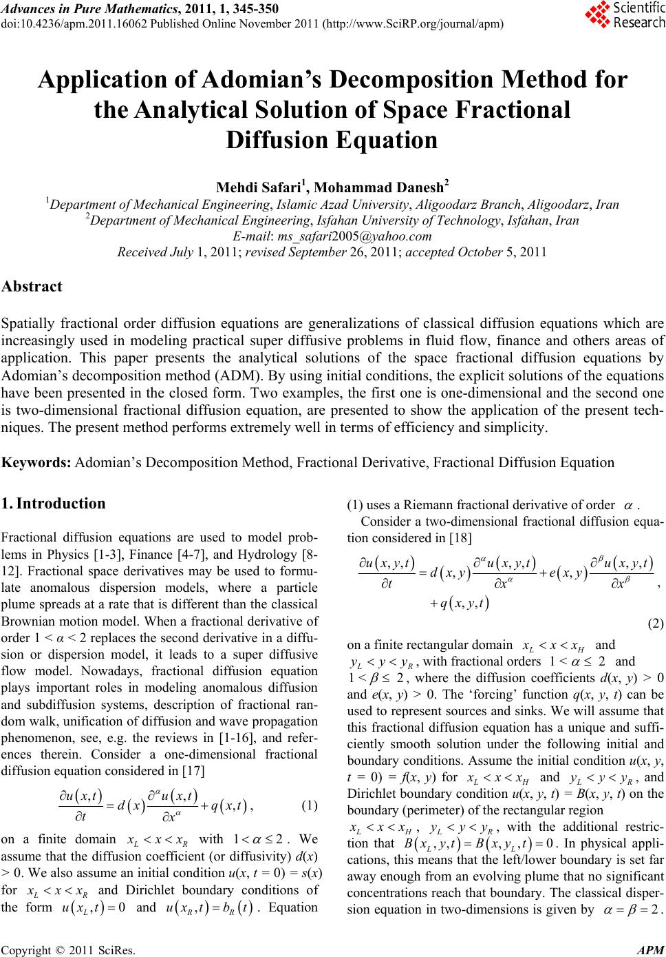