International Journal of Geosciences, 2011, 2, 476-483
doi:10.4236/ijg.2011.24050 Published Online November 2011 (http://www.SciRP.org/journal/ijg)
Numerical Modelling of the Topographic Wetness Index:
An Analysis at Different Scales
Anderson Luis Ruhoff1,2, Nilza Maria Reis Castro1, Alfonso Risso1
1Instituto de Pesquisas Hidraulicas, Universidade Federal do Rio Grande do Sul, Porto Alegre, Brazil
2Instituto de Ciências Humanas e da Informação, Universidade Federal do Rio Grande, Rio Grande, Brazil
Received September 13, 2011; revised October 15, 2011; accepted November 6, 2011
Abstract
A variety of landscape properties have been modeled successfully using topographic indices such as topog-
raphic wetness index (TWI), defined as ln(a/tanβ), where a is the specific upslope area and β is the surface
slope. In this study, 25 m spatial resolution from digital elevation models (DEM) data were used to investi-
gate the scale-dependency of TWI values when converting DEMs to 50 and 100 m. To investigate the impact
of different spatial resolution, the two lower resolution DEMs were interpolated to the original 25 m grid size.
In addition, to compare different flow-direction algorithms, a second objective was to evaluate differences in
spatial patterns. Thus the values of TWI were compared in two different ways: 1) distribution functions and
their statistics; and 2) cell by cell comparison of DEMs with the same spatial resolution but different flow-
directions. As in previous TWI studies, the computed specific upstream is smaller, on average, at higher
resolution. TWI variation decreased with increasing grid size. A cell by cell comparison of the TWI values of
the 50 and 100 m DEMs showed a low correlation with the TWI based on the 25 m DEM. The results
showed significant differences between different flow-diretction algorithms computed for DEMs with 25, 50
and 100 m spatial resolution.
Keywords: Resolution, DEM, Grid Size, Wetness Index
1. Introduction
Widely available digital elevation models (DEMs), to-
gether with corresponding tools for spatial analysis, have
found extensive use in the development of research in
many areas of the environmental sciences, including ag-
riculture, hydrology, ecology, geography and branches of
engineering using topographically-dependent variables.
The tools for digital elevation modeling [1-4, among
others] contain various options for the analysis of topog-
raphical attributes, such as algorithms for extracting
drainage networks [5-7], topographic indices [8], indices
of sediment transport capacity [9] and erosive potential
[9].
The most common sources of data for digital elevation
modeling are [10]: topographic bases with isolines and
points denoting maxima and minima, and transformed
field surveys undertaken, for example, with the use of
GPS, photogrammetry, stereoscopy from remote sensing
and radar interferometry, given in regular grid structures,
triangular grids and isoline nets [9].
Data are generated at different scales and spatial reso-
lutions. Quantities derived from topographic data need to
take account of the spatial limits imposed by the respec-
tive scales. At present, a number of spatial resolutions
are available for public use. Higher spatial resolutions
are obtained from photogrammetry and laser profiling,
while coarser spatial resolutions are freely available
through the Shuttle Radar Topographic Mission (SRTM)
[11]. The accuracy of data generated at different spatial
resolutions depends exclusively on how closely a calcu-
lated measure lies to its true value: the reliability of the
data is therefore linked to its accuracy. In this context,
the higher the spatial resolution of a DEM, the greater is
the tendency to accuracy. When analyzing data from a
DEM, a fundamental step is the evaluation of the preci-
sion of the derived data; the user must know how trust-
worthy his derived data is.
A number of authors have studied the effects of spatial
resolution on topographic data derived from DEMs, in-
cluding topographic derivatives of the first, second and
third orders [10,11], effects of spatial resolution in mod-

477 A. L. RUHOFF ET AL.
els for the direction of flow and accumulated overland
flow [12] and variations in the topographic index [13,
14].
A diagram relating the information in DEMs to hy-
drological information shows a qualitative and quantita-
tive decrease in hydrological information with reduction
in spatial resolution of DEMs [10]. Two situations can
determine the quality of hydrological information in high
resolution models: 1) the topography controls the hydro-
logical flows, giving an increase in hydrological infor-
mation; 2) soil characteristics determine the preferred
hydrological pathways, and in this case there is no in-
crease in hydrological information.
In this context, we attempted to evaluate the effects of
different flow-direction algorithms and spatial resolu-
tions on the TWI. The analysis of the scale effect on to-
pographic parameters in the drainage basin of the Po-
tiribu River [15] helps develop an understanding of their
magnitude and the way in which indices, such as soil
saturation, are affected.
2. Materials and Methods
2.1. The Potiribu River Basin
The study area lies within the Taboão River basin which
drains to the Potiribu River, lying to the northwest of the
Brazilian State of Rio Grande do Sul. The area is repre-
sentative of the basaltic plateau of the River Paraná basin
(Figure 1) where basaltic outflows extend over an area
of about 230,000 km2 [16]. The Potiribu River is a tribu-
tary of the Rio Ijuí, itself a left-bank tributary of the
River Uruguay. The total area of the Potiribu River basin
is 563 km² and consists of a number of nested sub-basins
monitored as part of the Potiribu Project. Physical char-
acteristics of these nested sub-basins are given in Table
1.
Altitude varies between 320 and 700 m. The relief is
undulating with gentle slopes between 3% and 15%.
Soils are fairly wet and well-developed as a consequence
of the abundant rainfall regime. Soils can be classified as
purple and dark-red latosol. Despite high clay content
(with percentages of clay in excess of 60%), there is a
well-developed drainage network as a result of soil
macropores [17].
The climate of the Potiribu River basin is classified as
Cfa: a mild, mesothermic and very damp climate with no
well-defined dry season. In this classification, mean
maximum temperatures are greater than 22˚C and mean
minimum temperatures are between –3˚C and 18˚C. Mean
temperatures in the region fluctuate between 18˚C and
19˚C, with July the coldest month (13˚C - 14˚C) and
January the hottest (24˚C). The mean maximum tempera-
ture is about 32˚C and the mean minimum about 8˚C.
Rainfall is determined by the interaction of large air
masses [15] resulting from: 1) turbulent southerly air
currents associated with polar anticyclone activity,
termed the polar front. This polar front occurs fairly
regularly with periodicity between 4 and 10 days, and is
accompanied by rainfall events that are generally long
and of moderate intensity, lingering for several con-
secutive days; 2) turbulent westerly currents associated
with lines of tropical that cross the Southern Region from
the middle of spring to the mid-October. Depressions are
induced by small tropical anticyclones of Amazonia.
These currents give rise to thunderstorms and convective
rainfall that is generally intense but of short duration.
Researchers at the Institute of Hydraulic Research [15,
Figure 1. Position of the Potiribu River basin in Brazil. The
broken line marks the limit of the basaltic plateau of the
Parana River basin.
Table 1. Physical characteristics of nested basins monitored by the Potiribu Project.
Basin Anfiteatro Donato Turcato Rincão Taboão Potiribu
Area (km2) 0.125 1.10 19.5 16.8 105 563
Perimeter (km) 1.42 4.54 17.9 17.4 47.5 115
Altitude range (m) 38.0 81.9 119.5 115.5 154.3 205.3
Slope index (m/km) 92.3 51.2 22.1 19.5 8.5 4.5

A. L. RUHOFF ET AL.
478
17,18] have monitored the Potiribu River basin with hy-
dro-sedimentological studies at a number of spatial and
time scales since the end of the 1980s. The research has
been supported by the Federal University of Rio Grande
do Sul (UFRGS), in collaboration with other research
institutions (ORSTOM-France, CNPq-Brazil, FAPERGS-
Brazil and FINEP-Brazil). The broad aim of the research
is to get a better understanding and description of hydro-
sedimentological processes at different spatial and time-
scales in a region of intense agricultural activity.
2.2. Methodology
The effects of different spatial resolutions on TWI have
been assessed by means of histograms, descriptive statis-
tics and regression analysis. The DEM with 25 m spatial
resolution was obtained by aerial photogrammetry; that
at 50 m resolution by digitizing contours of topographic
maps [19], and that at 100 m by resampling of data from
the Shuttle Radar Topographic Mission (SRTM) [22].
Indices derived from the DEMs were obtained using dif-
ferent algorithms to determine flow direction: 1) D8 [21],
2) DMF [22] and 3) D [23].
The TWI, given by Equation (1), defines areas of
saturated soil typically found in geomorphologically
convergent segments, where a is the area of specific con-
tribution based on flow-direction (summed over the area
upstream of the cell) and β is surface slope. It is deter-
mined from the flow direction and accumulated runoff.

ln tanTWI a

 (1)
The specific contributing area is related to the concept
of accumulated runoff and takes into account the com-
plexities of hill-slope form. The curvature of slopes both
in the plane and in profile effectively determines the hy-
dro-sedimentological behavior of erosive processes. It is
defined as the accumulated drainage area divided by the
width of the downstream contributing area (m2·m–1). In
the case of convex slopes for which accumulated flow is
divergent, the specific contributing area tends to dimin-
ish. For concave slopes, the specific contributing area
tends to increase, giving rise to a rapid increase in accu-
mulated downstream flow, defined as a specific contrib-
uting area [24].
In the D8, the flow directions are in the form of a
regular grid in which each cell’s value corresponds to
one of the eight possible directions. Obtaining the direc-
tion of flow for each pixel to one of its eight neighbors
can be done automatically, based on the difference in
level between them, weighted by distance. Thus a value
is attached to each pixel indicating one of the eight flow
directions. Following the flow directions, the number of
upslope cells is calculated which drain to a downslope
cell, so that the accumulated runoff is calculated.
However, the flow patterns from cell to cell are almost
never as simple, since a cell can receive flows from sev-
eral cells, so that the accumulated flow may be trans-
ferred to several other cells [25]. Therefore a proposed
multiple flow-direction algorithm (DMF) [22], in which
the flow transferred to each downslope cell is propor-
tional to the product of the distance over which flow is
accumulated and a geometrical weighting factor which
depends on the flow direction.
Since the D8 deals best with surface flow largely con-
centrated in the main channel, and the DMF deals with
dispersed surface flow, an algorithm with an infinite
number of possible flow directions was proposed [23], to
overcome the limitations of both D8 and DMF. The D
gives an unlimited number of flow directions using tri-
angular facets in a 3 × 3 pixel window. Thus the flow
distribution is proportioned amongst downslope pixels
according to the slope of each triangular facet. For a hy-
pothetical conical surface, there is a concentration of
surface flow in the D8, and a substantial dispersion of
surface flow in the DMF. The D gives no substantial
spreading of surface flow nor a concentration of flow in
a single main channel, such as that occurring in the D8
and DMF.
3. Results and Discussion
The analyses reported here have two distinct aspects: 1)
the effect of the flow-direction algorithm and 2) the ef-
fects of different spatial resolutions. At 25 m resolution,
along the main channel and its tributaries and in these
areas the highest values were found. Values found on the
slopes were much smaller than those in the main chan-
nels. When the DMF was used, TWI showed a much
smoother behavior than that found using the D8. The
main channels could be seen but the tributaries could no
longer be distinguished, having values very similar to
those on the hill-slopes. The largest values found in the
main channels when the DMF was used were smaller than
those given in the main channels by the D8 algorithm.
The TWI generated by the D gave results very similar
to those given by the D8, although tributaries to the main
channel were less in evidence as a consequence of the
considerably greater dispersion of runoff. Descriptive
statistics of indices generated by the three flow-direction
algorithms were very similar, although the summary sta-
tistics increased with the pixel size (Table 2). The fre-
quency distribution shows significant differences be-
tween the flow-direction algorithms (p-value < 0.05) and
between spatial resolutions (p-value < 0.05) (Figure 2).
For indices generated by the D8, the mean gradually
increases from 7.45 to 8.35 for resolutions 25 and 100 m

479 A. L. RUHOFF ET AL.
Table 2. Descriptive statistics of topographic indices generated by simple flow algorithm (D8), multiple-flow algorithm (DMF)
and triangular facets flow algorithm (D∞), at spatial resolutions of 25, 50 and 100 m.
Resolution 25 m Resolution 50 m Resolution 100 m
D8 DMF D D8 DMF D D8 DMF D
Mean 7.45 7.86 7.45 7.84 8.14 7.95 8.35 8.54 8.41
S. Deviation 1.38 1.16 1.38 1.37 1.20 1.29 1.31 1.20 1.27
Minimum 4.25 4.65 4.27 5.11 5.59 5.27 6.25 6.70 6.37
1st quartile 6.59 7.18 6.59 6.99 7.45 7.19 7.51 7.80 7.61
Median 7.25 7.61 7.25 7.54 7.82 7.60 7.97 8.14 8.01
3rd quartile 7.94 8.15 7.94 8.23 8.34 8.21 8.72 8.77 8.73
Maximum 17.85 17.94 19.86 19.67 18.66 19.20 16.18 16.16 17.41
Figure 2. Frequency distribution of topographic wetness index (TWI) for different spatial resolutions (25, 50 and 100 m) using
8, DMF and D∞ flow-direction algorithms. D

A. L. RUHOFF ET AL.
480
respectively. Minimum values vary between 4.25 and
6.25, while the lower quartile varies between 6.59 and
7.51 and the upper quartile between 7.94 and 8.72 at
resolutions 25 and 100 m. For the DMF, the mean shows
increases from 7.86 to 8.54 at resolutions from 25 to 100
m respectively. Minimum values vary between 4.65 and
6.70, while the lower quartile varies from 7.18 to 7.80
and the upper quartile from 8.15 to 8.77 at resolutions
from 25 to 100 m. For the D, the mean shows increases
from 7.45 to 8.41, at resolutions from 25 to 100 m, re-
spectively. Minimum values vary between 4.27 and 6.37,
while the lower quartile varies from 6.59 to 7.61 and the
upper quartile from 7.94 to 8.73, at resolutions from 25
to 100 m.
Increases in descriptive statistics are therefore found at
spatial resolutions from 25 to 100 m. Minimum values,
lower quartile, mean, median and upper quartile increase
as pixel size increases (as DEM resolution decreases).
Taking the 25 m spatial resolution as the most represen-
tative of TWI, the D8 gives increases of 5.23% and
12.08% in the mean value of indices generated at resolu-
tions 50 and 100 m respectively. For the DMF, increases
are 3.68% and 8.65% at resolutions 50 and 100 m, while
for the D the increases are 6.71% and 12.88%.
The greatest maximum values were found in indices
generated at 50 m spatial resolution, whilst the smallest
maxima values were found at 100 m resolution. For the
D8, variations from 10.20% to –10.36% were found
when comparing resolutions 50 and 100 m respectively,
with the 25 m resolution. For the DMF, these changes
were between 4.01% and –9.93%, respectively, and for
the D, between –3.32% and –12.33%. The magnitude
of these variations in maximum values of TWI is proba-
bly a consequence of smoothing the DEM and the slope
indices, as for each slope segment at 100m resolution
there are 2 and 4 slope segments at resolutions 50 and 25
m respectively.
A pixel-by-pixel comparison of root mean square error
(RMSE) at the different spatial resolutions shows where
the greatest variations in scale effects occur. A bilinear
interpolator was used to resample the topographic indices
from 50 and 100 m to 25 m. The greatest differences are
found along the main channel and its tributaries, whilst
differences on hill-slopes are smaller. In the case of D8,
the RMSE between 25 and 50 m was 0.96 ± 1.42 and
between 25 and 100 m, the RMSE was 1.44 ± 1.60. For
the D, the RMSE was 0.92 ± 1.30 and 1.43 ± 2.51 at
spatial resolutions from 25 to 50 m and 25 to 100 m, re-
spectively. Considering DMF, the RMSE between 25 and
50 m, and between 25 and 100 m, were smaller than the
differences generated by the D8 and D.
It can be concluded, from these analyses at different
resolutions, that the greatest differences are found be-
tween indices generated at 25 and 100 m resolutions us-
ing the D8 and D, since the greatest flows are propa-
gated in the main channels. In this context, indices gen-
erated by the multiple-flow DMF show differences that
are substantially smaller than those given by the D8 and
D algorithms, mainly as a result of the way in which
flow is distributed. Figure 3 shows a box-plot diagram
Figure 3. Ranges of root mean square error (RMSE) between spatial resolutions from 25 to 50 m (1) and from 25 to 100 m (2)
for TWI generated by the D8 algorithm; from 25 to 50 m (3) and from 25 to 100 m (4) using DMF algorithm; from 25 to 50 m
5) and from 25 to 100 m (6) using D∞ algorithm. (

481 A. L. RUHOFF ET AL.
of the RMSE between 25 and 50 m resolutions and 25
and 100 m spatial resolution, for TWI generated by the
D8, DMF e D algorithms. An analysis of the dispersion
amongst resampled data shows that there is not correla-
tion between indices generated from the different spatial
resolutions (Figure 4).
4. Concluding Remarks
The spatial resolution of DEMs is a major influence on
the values of indices such as topographic wetness index,
derived from numerical models. Equally, determination
of direction of flow and of specific contributing area de-
pends on the flow-direction algorithm used. Algorithms
such as the simple flow D8, the multiple-flow DMF and
the algorithm based on triangular facets such as D, can
give rise to quite different results.
From the analyses using different algorithms for flow
direction, it can be concluded that 1) the D8 concentrated
runoff along the main channel, whilst the DMF algorithm
gave dispersal of runoff, and the D gave intermediate
results; 2) descriptive statistics showed subtle differences,
Figure 4. Correlation of the topographic wetness index (TWI) between different spatial resolutions.

A. L. RUHOFF ET AL.
482
mainly in terms of minimum values, means, lower quar-
tile and the median.
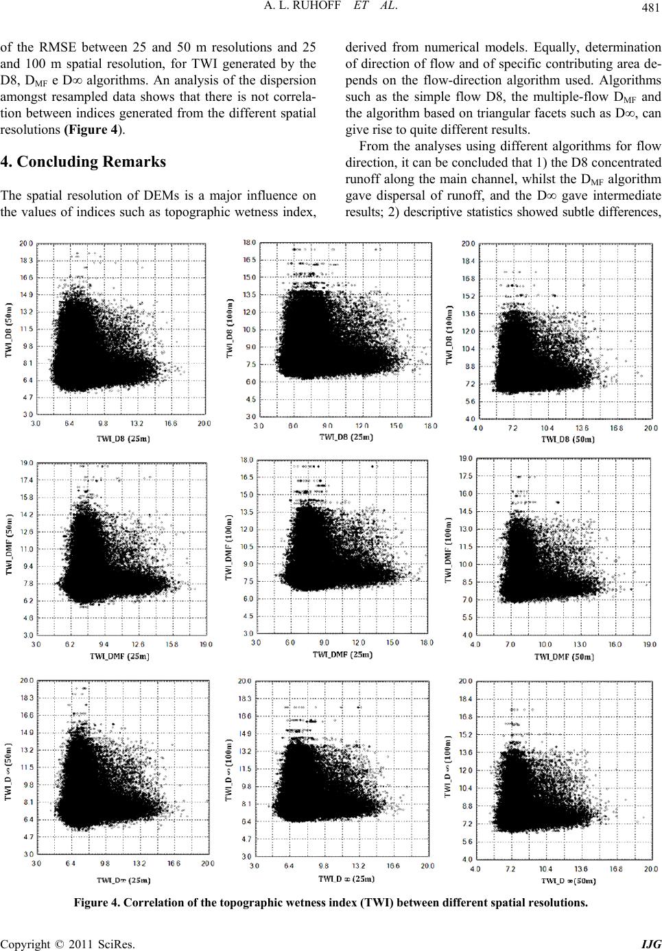
Analyses of the effects of different spatial resolutions
showed significant variation between descriptive statis-
tics, with quite different results. Little correlation was
found between indices at resolutions 25, 50 and 100 m,
in agreement with other results [14]. However in more
than 75% of cases the differences were quite subtle, with
differences in TWI lower than two points. A pixel-by-
pixel analysis showed that the greatest differences oc-
curred mostly along the main channel, independently of
the algorithm used to determine flow direction. There
was also greater concentration of differences along tribu-
taries of the main channel, when the D8 and D were
used. Differences in the topographic index tended to be
smaller in the headwater areas of the drainage network
and on hillslopes, where runoff is smaller.
It can be concluded from the results that there are
many differences between values of TWI generated at
different spatial resolutions and by different flow-direc-
tion algorithms, but it is not clear that results obtained at
more detailed spatial resolutions are necessarily better.
The effects of scale can become more accentuated or less
so, depending on the topographic influences on hydro-
logic processes.
5. References
[1] J. P. Wilson and J. C. Gallant, “TAPES-G: A Grid-Based
Terrain Analysis Program for the Environmental Sci-
ences,” Computers e Geosciences, Vol. 22, No. 7, 1996,
pp. 713-722.
doi:10.1016/0098-3004(96)00002-7
[2] J. Blaszcynski, “Landform Characterization with GIS,”
Photogrammetric Engineering and Remote Sensing, Vol.
63, 1997, pp. 183-191.
[3] J. R. Eastman, “Idrisi Andes—Guide to GIS and Image
Processing,” Clark University, Worcester, 2006..
[4] J. Schauble, “Hydrotools for Arcview,” Institute of Ap-
plied Geosciences, Technical University of Darmstadt,
Darmstadt, 2000.
[5] S. K. Jenson and J. O. Domingue, “Extracting Topog-
raphic Structure from Digital Elevation Data for Geo-
graphic Information System Analysis,” Photogrammetric
Engineering and Remote Sensing, Vol. 54, 1988, pp.
1593-1600.
[6] D. G. Tarboton, R. L. Bras and I. Rodriguez-Iturbe, “On
the Extraction of Channel Networks from Digital Eleva-
tion Data,” Hydrological Processes, Vol. 5, No. 1, 1991,
pp. 81-100. doi:10.1002/hyp.3360050107
[7] O. Planchon and F. Darboux, “A Fast, Simple and Versa-
tile Algorithm to Fill the Depressions of Digital Elevation
Models,” Catena, Vol. 46, No. 2-3, 2001, pp. 159-176.
[8] K. J. Beven and M. J. Kirkby, “A Physically Based Vari-
able Contributing Area Model of Basin Hydrology,” Hy-
drological Sciences Bulletin, Vol. 24, No. 1, 1979, pp.
43-69. doi:10.1080/02626667909491834
[9] I. D. Moore, R. B. Grayson and A. R. Ladson, “Digital
Terrain Modelling: A Review of Hydrological, Geomor-
phological, and Biological Applications,” Hydrological
Processes, Vol. 5, No. 1, 1991, pp. 3-30.
doi:10.1002/hyp.3360050103
[10] J. P. Wilson and J. C. Gallant, “Terrain Analysis: Princi-
ples and Applications,” John Wiley & Sons Inc., New
York, 2000.
[11] S. Kienzle, “The Effects of DEM Raster Resolution on
First Order, Second Order and Compound Terrain Deri-
vates,” Transactions in GIS, Vol. 8, No. 1, 2004, pp. 83-
111. doi:10.1111/j.1467-9671.2004.00169.x
[12] M. S. Horritt and P. D. Bates, “Predicting Floodplain
Inundation: Raster-Based Modelling versus the Finite-
Element Approach,” Hydrological Processes, Vol. 15,
No. 5, 2001, pp. 825-842. doi:10.1002/hyp.188
[13] A. Gunter, J. Seibert and S. Uhlenbrook, “Modeling Spa-
tial Patterns of Saturated Areas: An Evaluation of Dif-
ferent Terrain Inideces,” Water Resources Research, Vol.
40, 2004, pp. 1-19.
[14] R. Sorensen and J. Seibert, “Effects of DEM Resolution
on the Calculation of topographical indices: TWI and Its
Components,” Journal of Hydrology, Vol. 347, No. 1-2,
2007, pp. 79-89. doi:10.1016/j.jhydrol.2007.09.001
[15] N. M. R. Castro, A. V. Auzet, P. Chevallier and J. C.
Leprun, “Land Use Change Effects on Runoff and Ero-
sion from Plot to Catchment Scale on the Basaltic Plateau
of Southern Brazil,” Hydrological Processes, Vol. 13, No.
11, 1999, pp. 1621-1628.
doi:10.1002/(SICI)1099-1085(19990815)13:11<1621::AI
D-HYP831>3.0.CO;2-L
[16] A. L. O. Borges and M. P. Bordas, “Escolha de Bacias
Representativas e Experimentais Para o estudo da erosão
no Planalto Basáltico Sul-Americano,” Congresso brasileiro
e encontro nacional de pesquisa sobre conservação do
solo, Londrina, 1990.
[17] N. M. R. Castro, “Ruissellement et érosion sur des
bassins versants de grande culture du plateau basaltique
du sud du Brésil (Rio Grande do Sul),” Tese (Doutorado),
Université Louis Pasteur, Strasbourg, 1996.
[18] P. Chevallier, “As precipitações na região de Cruz Alta e
Ijuí (RS-Brasil),” Caderno de Recursos Hídricos, Vol. 24,
1991, pp. 1-24
[19] M. Eineder, A. Roth, R. Bamler and B. Rabus, “The
Shuttle Radar Topography Mission—A New Class of
Digital Elevation Models Acquired by Spaceborne Ra-
dar,” ISPRS Journal of Photogrammetry e Remote Sens-
ing, Vol. 57, No. 4, 2003, pp. 241-262.
doi:10.1016/S0924-2716(02)00124-7
[20] J. F. O’Callaghan and D. M. Mark, “The Extraction of
Drainage Networks from Digital Elevation Data,” Com-
puter Vision, Graphics, and Image Processing, Vol. 28,
1984, pp. 328-344.
[21] P. F. Quinn, K. J. Beven and R. Lamb, “The ln(a/tanβ)

483 A. L. RUHOFF ET AL.
Index: How to Calculate it and How to Use it within the
Topmodel Framework,” Hydrological Processes, Vol. 9,
No. 42, 1995, pp. 161-182. doi:10.1002/hyp.3360090204
[22] D. G. Tarboton, “A New Method for the Determination of
Flow Directions and Upslope Areas in Grid Digital Ele-
vation Models,” Water Resources Research, Vol. 33, No.
2, 1997, pp. 309-319. doi:10.1029/96WR03137
[23] C. A. Onstad and D. L. Brakensiek, “Watershed Sim-
ulation by the Stream Path Analogy,” Water Resources
Research, Vol. 4, No. 5, 1968, pp. 965-971.
doi:10.1029/WR004i005p00965
[24] C. D. Renno, “Sistema de análise e simulação hidrológica
aplicado a bacias hidrográficas,” Tese (Doutorado em
Sensoriamento Remoto), Instituto Nacional de Pesquisas
Espaciais, São José dos Campos, 2003.