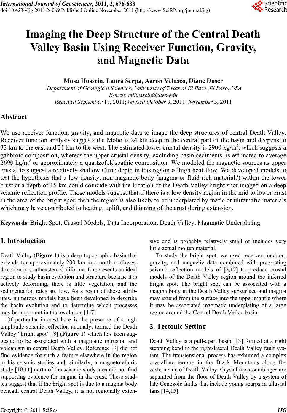International Journal of Geosciences, 2011, 2, 676-688
doi:10.4236/ijg.2011.24069 Published Online November 2011 (http://www.SciRP.org/journal/ijg)
Imaging the Deep Structure of the Central Death
Valley Basin Using Receiver Function, Gravity,
and Magnetic Data
Musa Hussein, Laura Serpa, Aaron Velasco, Diane Doser
1Department of Geol o gi cal Sciences, University of Texas at El Paso, El Paso, USA
Received September 17, 2011; revised October 9, 2011; November 5, 2011
Abstract
We use receiver function, gravity, and magnetic data to image the deep structures of central Death Valley.
Receiver function analysis suggests the Moho is 24 km deep in the central part of the basin and deepens to
33 km to the east and 31 km to the west. The estimated lower crustal density is 2900 kg/m3, which suggests a
gabbroic composition, whereas the upper crustal density, excluding basin sediments, is estimated to average
2690 kg/m3 or approximately a quartzofeldspathic composition. We modeled the magnetic sources as upper
crustal to suggest a relatively shallow Curie depth in this region of high heat flow. We developed models to
test the hypothesis that a low-density, non-magnetic body (magma or fluid-rich material?) within the lower
crust at a depth of 15 km could coincide with the location of the Death Valley bright spot imaged on a deep
seismic reflection profile. Those models suggest that if there is a low density region in the mid to lower crust
in the area of the bright spot, then the region is also likely to be underplated by mafic or ultramafic materials
which may have contributed to heating, uplift, and thinning of the crust during extension.
Keywords: Bright Spot, Crustal Models, Data Incorporation, Death Valley, Magmatic Underplating
1. Introduction
Death Valley (Figure 1) is a deep topographic basin that
extends for approximately 200 km in a north-northwest
direction in southeastern California. It represents an ideal
region to study basin evolution and structure because it is
actively deforming, there is little vegetation, and the
sedimentation rates are low. As a result of these attrib-
utes, numerous models have been developed to describe
the basin evolution and to determine which processes
may be important in that evolution [1-7]
Of particular interest here is the presence of a high
amplitude seismic reflection anomaly, termed the Death
Valley “bright spot” [8] (Figure 1) which has been sug-
gested to be associated with a magmatic intrusion and
volcanism in central Death Valley. Reference [9] did not
find evidence for such a feature elsewhere in the region
in his seismic studies and, similarly, a magnetotelluric
study [10,11] north of the seismic study area did not find
supporting evidence for magma in the crust. These stud-
ies suggest that if the bright spot is due to a magma body
beneath central Death Valley, it is not regionally exten-
sive and is probably relatively small or includes very
little actual molten material.
To study the bright spot, we used receiver function,
gravity, and magnetic data combined with preexisting
seismic reflection models of [2,12] to produce crustal
models of the Death Valley region around the inferred
bright spot. The bright spot can be associated with a
magma body in the Death Valley subsurface and magma
may extend from the surface into the upper mantle where
it may be associated magmatic underplating of a large
region around the Central Death Valley basin.
2. Tectonic Setting
Death Valley is a pull-apart basin [13] formed at a right
stepping bend in the right-lateral Death Valley fault sys-
tem. The transtensional process has exhumed a complex
crystalline terrane in the Black Mountains along the
eastern side of Death Valley. Crystalline assemblages are
separated from the floor of Death Valley by a system of
late Cenozoic faults that include young scar ps in alluvial
fans [14,15].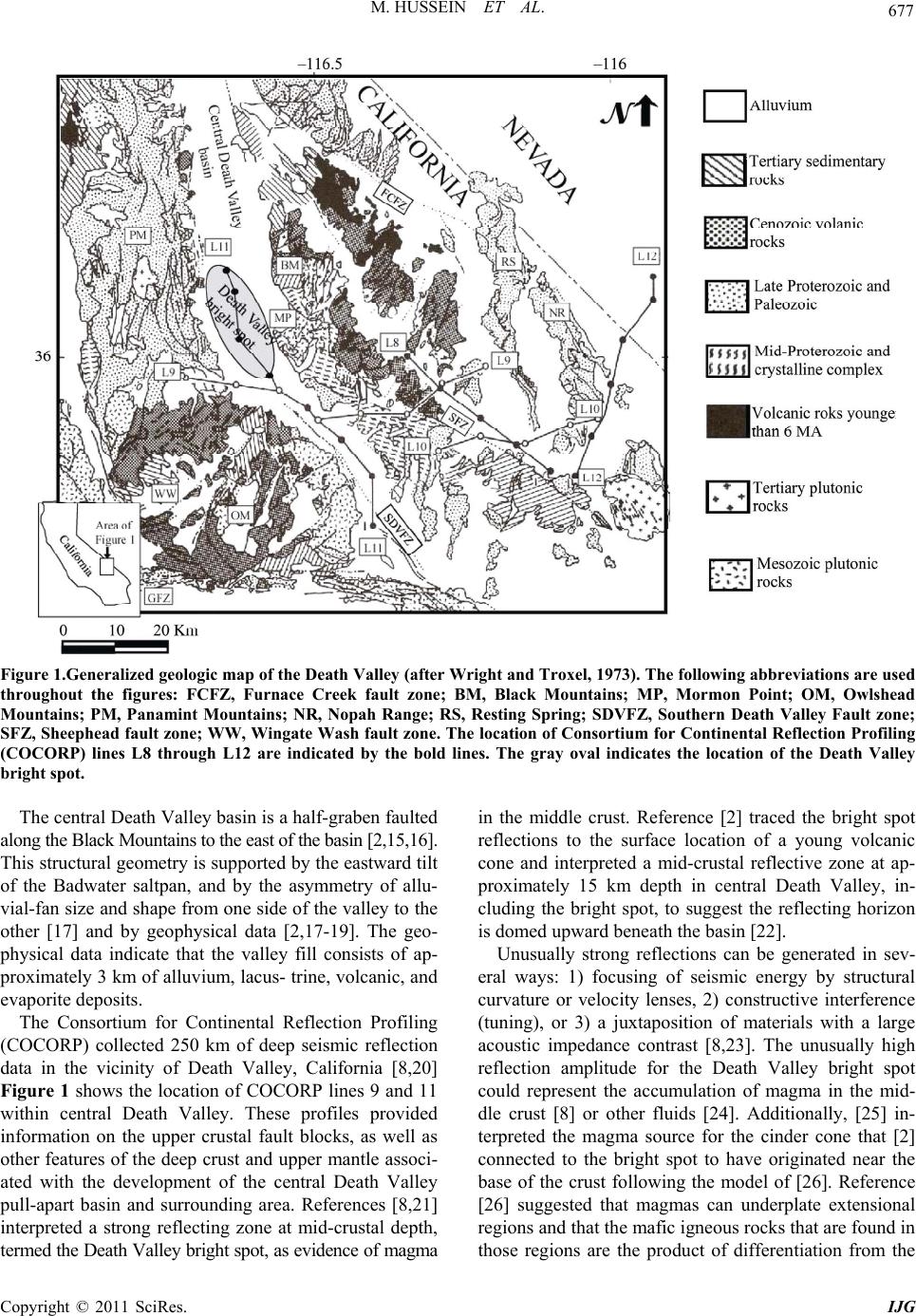

M. HUSSEIN ET AL.
677
Figure 1.Generalized geologic map of the Death Valley (after Wright and Troxel, 1973). The following abbreviations are used
throughout the figures: FCFZ, Furnace Creek fault zone; BM, Black Mountains; MP, Mormon Point; OM, Owlshead
Mountains; PM, Panamint Mountains; NR, Nopah Range; RS, Resting Spring; SDVFZ, Southern Death Valley Fault zone;
SFZ, Sheephead fault zone; WW, Wingate Wash fault zone. The location of Consortium for Continental Reflection Profiling
(COCORP) lines L8 through L12 are indicated by the bold lines. The gray oval indicates the location of the Death Valley
bright spot.
The central Death Valley basin is a half-graben faulted
along the Black Mountains to the east of the basin [2,15,16].
This structural geometry is supported by the eastward tilt
of the Badwater saltpan, and by the asymmetry of allu-
vial-fan size and shape from one side of the valley to the
other [17] and by geophysical data [2,17-19]. The geo-
physical data indicate that the valley fill consists of ap-
proximately 3 km of alluvium, lacus- trine, vo lcanic, and
evaporite deposits.
The Consortium for Continental Reflection Profiling
(COCORP) collected 250 km of deep seismic reflection
data in the vicinity of Death Valley, California [8,20]
Figure 1 shows the location of COCORP lines 9 and 11
within central Death Valley. These profiles provided
information on the upper crustal fault blocks, as well as
other features of the deep crust and upper mantle associ-
ated with the development of the central Death Valley
pull-apart basin and surrounding area. References [8,21]
interpreted a strong reflecting zone at mid-crustal depth,
termed the Death Valley bright spot, as evidence of magma
in the middle crust. Reference [2] traced the bright spot
reflections to the surface location of a young volcanic
cone and interpreted a mid-crustal reflective zone at ap-
proximately 15 km depth in central Death Valley, in-
cluding the bright spot, to suggest the reflecting horizon
is domed upward beneath the basin [22].
Unusually strong reflections can be generated in sev-
eral ways: 1) focusing of seismic energy by structural
curvature or velocity lenses, 2) constructive interference
(tuning), or 3) a juxtaposition of materials with a large
acoustic impedance contrast [8,23]. The unusually high
reflection amplitude for the Death Valley bright spot
could represent the accumulation of magma in the mid-
dle crust [8] or other fluids [24]. Additionally, [25] in-
terpreted the magma source for the cinder cone that [2]
connected to the bright spot to have originated near the
base of the crust following the model of [26]. Reference
[26] suggested that magmas can underplate extensional
regions and that the mafic igneous rock s that are found in
those regions are the product of differentiation from the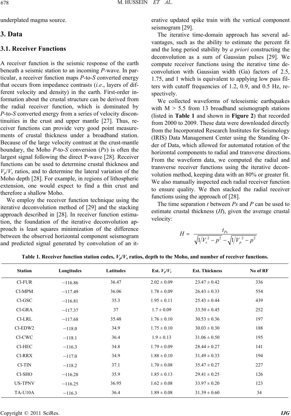

M. HUSSEIN ET AL.
678
underplated magma source.
3. Data
3.1. Receiver Functions
A receiver function is the seismic response of the earth
beneath a seismic station to an incoming P-wave. In par-
ticular, a receiver function maps P-to-S converted energy
that occurs from impedance contrasts (i.e., layers of dif-
ferent velocity and density) in the earth. First-order in-
formation about the crustal structure can be derived from
the radial receiver function, which is dominated by
P-to-S converted energy from a series of velocity discon-
tinuities in the crust and upper mantle [27]. Thus, re-
ceiver functions can provide very good point measure-
ments of crustal thickness under a broadband station.
Because of the large velocity contrast at the crust-mantle
boundary, the Moho P-to-S conversion (Ps) is often the
largest signal following the direct P-wave [28]. Receiver
functions can be used to determine crustal thickness and
Vp/Vs ratios, and to determine the lateral variation of the
Moho depth [28]. For example, in regions of lithospheric
extension, one would expect to find a thin crust and
therefore a shallow Moho.
We employ the receiver function technique using the
iterative deconvolution method of [29] and the stacking
approach described in [28]. In receiver function estima-
tion, the foundation of the iterative deconvolution ap-
proach is least squares minimization of the difference
between the observed horizontal component seismogram
and predicted signal generated by convolution of an it-
erative updated spike train with the vertical component
seismogram [29].
The iterative time-domain approach has several ad-
vantages, such as the ability to estimate the percent fit
and the long period stability by a priori constructing the
deconvolution as a sum of Gaussian pulses [29]. We
compute receiver functions using the iterative time de-
convolution with Gaussian width (Ga) factors of 2.5,
1.75, and 1 which is equivalent to applying low pass fil-
ters with cutoff frequencies of 1.2, 0.9, and 0.5 Hz, re-
spectively.
We collected waveforms of teleseismic earthquakes
with M > 5.5 from 13 broadband seismograph stations
(listed in Table 1 and shown in Figure 2) that recorded
from 2000 to 2009. These data were downloaded directly
from the Incorporated Research In stitutes for Seismology
(IRIS) Data Management Center using the Standing Or-
der of Data, which allowed for automated rotation of the
horizontal components to radial and transverse directions.
From the waveform data, we computed the radial and
transverse receiver functions using the iterative decon-
volution method, keeping data with an 80% or greater fit.
We also manually inspected each radial receiver function
to ensure quality. We then stacked the radial receiver
functions using the approach of [28].
The time separation t between Ps and P can be used to
estimate crustal thickness (H), given the average crustal
velocity:
22 22
11

 
Ps
sp
t
HVp Vp
Table 1. Receiver function station codes, Vp/Vs ratios, depth to the M oho, and number of receiver func tions.
Station Longitudes Latitudes Est. Vp/Vs Est. Thickness No of RF
Cl-FUR –116.86 36.47 2.02 ± 0.09 23.47 ± 0.42 336
Cl-MPM –117.49 36.06 1.78 ± 0.09 26.43 ± 0.33 554
Cl-GSC –116.81 35.3 1.95 ± 0.11 25.43 ± 0.44 439
Cl-GRA –117.37 37 1.7 ± 0.09 33.50 ± 0.45 252
Cl-LRL –117.68 35.48 1.76 ± 0.10 30.53 ± 0.36 197
Cl-EDW2 –118.0 34.9 1.75 ± 0.10 30.03 ± 0.30 188
Cl-CWC –118.1 36.4 1.9 ± 0.13 31.06 ± 0.50 195
Cl-HEC –116.3 34.8 1.79 ± 0.09 28.44 ± 0.27 141
Cl-RRX –117.0 34.9 1.88 ± 0.10 31.49 ± 0.33 194
Cl-TIN –118.2 37.1 1.70 ± 0.08 35.47 ± 0.27 227
Cl-SHO –116.28 35.9 1.85 ± 0.13 29.41 ± 0.25 126
US-TPNV –116.25 36.95 1.62 ± 0.08 33.97 ± 0.20 123
TA-U10A –116.3 36.4 1.89 ± 0.08 31.39 ± 0.60 34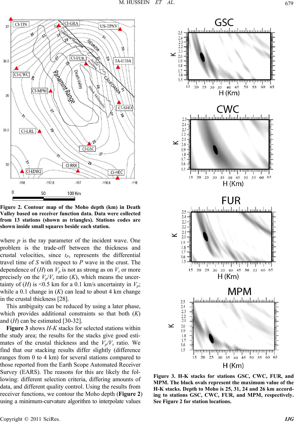

M. HUSSEIN ET AL.
679
Figure 2. Contour map of the Moho depth (km) in Death
Valley based on receiver function data. Data were collected
from 13 stations (shown as triangles). Stations codes are
shown inside small squares beside eac h station.
where p is the ray parameter of the incident wave. One
problem is the trade-off between the thickness and
crustal velocities, since tPs represents the differential
travel time of S with respect to P wave in the crust. The
dependence of (H) on Vp is not as strong as on Vs or more
precisely on the Vp/Vs ratio (K), which means the uncer-
tainty of (H) is <0.5 km for a 0.1 km/s uncertainty in Vp;
while a 0.1 change in (K) can lead to about 4 km change
in the crustal thickness [28].
This ambiguity can be reduced by using a later phase,
which provides additional constraints so that both (K)
and (H) can be estimated [30-32].
Figure 3 shows H-K stacks for selected stations within
the study area; the results for the stacks give good esti-
mates of the crustal thickness and the Vp/Vs ratio. We
find that our stacking results differ slightly (difference
ranges from 0 to 4 km) for several stations compared to
those reported from the Earth Scope Automated Receiver
Survey (EARS). The reasons for this are likely the fol-
lowing: different selection criteria, differing amounts of
data, and different quality control. Using the results from
receiver functions, we contour the Moho depth (Figure 2)
using a minimum-curvature algorithm to interpolate values
Figure 3. H-K stacks for stations GSC, CWC, FUR, and
MPM. The black ovals represent the maximum value of the
H-K stacks. Depth to Moho is 25, 31, 24 and 26 km acco rd-
ing to stations GSC, CWC, FUR, and MPM, respectively.
See Figure 2 for station locations.

M. HUSSEIN ET AL.
680
to a rectangular grid. Although no stations fall within
Death Valley, there is clear evidence that Moho depth
decreases toward the valley based on the trends from the
stations located closest to the valley. In particular, there
is a station (CI-FUR in Figure 2 and Table 1) near the
northern end of central Death Valley that clearly shows
the shallowest Moho at less than 24 km depth in the area.
Thus, the Moho appears to have a dome shape, with
Moho depth decreasing from approximately 31 km out-
side the Valley to 20 - 25 km in central Death Valley, as-
suming a relatively uniform rate of change from the areas
where the stations are located.
The Vp/Vs ratio (Table 1) ranges from 2 to 1.91 in
central Death Valley and from 1.85 to 1.73 in the other
areas. The major factor producing high Vp/Vs is the pla-
gioclase-rich mafic composition of the lower crust [33].
Reference [34] concluded that a low Vp velocity com-
bined with low Vp/Vs zones in the upper crust are caused
by the inclusion of H2O and that a low Vp velocity with
high Vp/Vs zones in the lower crust and the uppermost
mantle are caused by melt inclusions. That model sug-
gests the high Vp/Vs ratio in the lower crust is indicative
of a mafic lower crustal composition bu t we do not hav e an
independent measure of Vp to use to determine whether
there is magma in the crust.
3.2. Gravity and Aeromagnetic Data
We obtained gravity data from the University of Texas at
El Paso (UTEP) -Pan American Center of Earth and En-
vironmental Studies-(PACES) that is currently hosted at
the CYBER-ShARE Center of Excellence at UTEP
(http://www.research.utep.edu/paces). The gravity data
were merged from a variety of surveys and cover the U.S.
and the border region. The average error for this data set
ranges from 0.05 to 2mGal (Al-Douri, personal commu-
nication, 2009). Terrain corrections were calculated by
[35] of the U. S. Geological Survey (USGS) using a
digital elevation model and a technique based on the ap-
proach of [3 6] .
A Bouguer gravity correction was made using 2670
kg/m3 as the reduction density. We used 7,930 Bouguer
gravity points to create the Bouguer gravity anomaly
map (Figures 4 and 5). Aeromagnetic data were ob-
tained from the U.S. Geological Survey with a grid
spacing of 1 km [37]. We used a total of 36,342 digitized
aeromagnetic points to create the magnetic anomaly map
(Figure 6).
Figure 4. Bouguer anomaly map of the Death Valley area. The *marks a gravity low (–120 to –130 mGal), which coincides wit h
the Death Valley bright spot location. Large amplitude gravity anomalies are observed along the southern Death Valley fault
zone (SDVFZ) and to the southeast. Note the well defined alignment of anomalies along the Garlock fault zone. Solid lines
A-A` and B-B` show the location of the gravity profiles shown in Figures 8 and 9. The locations of the profiles were chosen to
illustrate the general crustal structure of the study area. FCFZ, Furnace Creek fault zone; SDVFZ, Southern Death Valley
Fault zone; GFZ, Garlock Fault Zone.

M. HUSSEIN ET AL.
681
Figure 5. Gravity stations location map, solids lines show location of gravity profiles shown in Figures 8 and 9. The study area
covered wit total of (7930) gravity measurements.
Figure 6. Aeromagnetic anomaly map of Death Valley area. The * is a magnetic low which coincides with the location of the
Death Valley bright spot. FCFZ, Furnace Creek fault zone; SDVF Z, Southern Death Valley Fault zone; GFZ, Garlock Fault
Zone.

M. HUSSEIN ET AL.
682
4. Model Development
We based our initial models on the seismic reflection
interpretations [2,8,12,18] and the receiver function data.
4.1. Bouguer Gravity Anomaly Map
The Bouguer gravity values decrease from –80 mGal in
the Black Mountains to –180 mGal to the west and nor th
(Figure 4) of the Black Mountains. Low gravity anoma-
lies are likely caused by unconsolidated sediments in the
basins, metasedimentary and granitic rocks, or by thicker
crust or some combination of these features. Thus, the
observation that the gravity values are significantly lower
over the Panamint Range than over the Black Mountains
is consistent with the interpretations [3,4,38] that the
Panamint Range is comprised primarily of upper crustal
rocks that have moved off the lower crustal rocks now
exposed in the Black Mountains.
Other features of interest are the continuity of the large
amplitude gravity and magnetic anomalies along the south-
ern Death Valley fault zone and into the Moj ave terrane and
the well defined alignment of anomalies along the Garlock
fault zone. The Panamint Range and the Northern Death
Valley fault zone are not as well defined by the potential
field data as are the anomalies associated with the Black
Mountains, southern Death Valley and Garlock fault
zones. One possible explanation for these observations is
that the Panamint Range and Northern Death Valley fault
zones are shallow features or, at least, they involve greater
thickness of upper crustal, low density materials than the
Black Mountains and southern Death Valley regions. On
the other hand, the Black Mountains and faults to the south
may represent more crustal scale features that could bring
high density mantle m aterials clos er to t he s urface lo cally.
The Death Valley bright spot (Figures 4 and 6) corre-
sponds to a gravity low (–120 to –130 mGal), which is
consistent with the interpretation by [8] of a deep magma
body. One concern is that the gravity low in central
Death Valley basin could be due to the basin sediment
material rather than deeper structures. To further explore
the source of this low gravity anomaly we modeled the
first 5 km of the crust in central and southern Death Val-
ley region using gravity and magnetic data with the
seismic data interpretation of [12] for line L9 (Figure 1).
The potential field model and comparison (Figure 7)
Figure 7. Comparison model of the first 5 km of the crust from velocity model of Louie et al. (1997) Reference [12], for
COCORP line 9-L9 (Figure 1), with density (D) and magnetic susceptibility (S) model in central and southern Death Valley.

M. HUSSEIN ET AL.
683
show a good match between the observed and calculated
gravity data.
This suggests the gravity and magnetic anomalies are
entirely due to the basin structure but it does not explain
why the COCORP seismic data show an anomaly at 15
km depth and why a young volcanic cinder con e exists in
the study area which is an indication of a magmatic ma-
terial in the crust, additionally all the material beneath an
observation site affects the gravity value. Thus, we chose
to explore the model possibilities further.
4.2. Crustal Models
Figure 4 shows the locations of two 2.5-dimensional
(2.5-D) crustal models (Figures 8 and 9) across the
bright spot constructed using a gravity and magnetic pro-
gram developed by [39] and further revised by [40] and
[41]. Gravity and magnetic values were extracted from
the grid at 2-km intervals. These values were then input
as observed data to the 2.5-D forward modeling program.
The modeled profiles illustrate the general deep structure
of the region and are not intended to reflect the detailed
surface geology. Where seismic data are available, we
have incorpora ted that infor mation into the models. In gen-
eral, gravity modeling produces non-unique results; how-
ever, we propose that by incorporating gravity, magnetic,
receiver function, and seismic reflecti on/re fracttio n data, we
can produce a well constrained model. Thus, as starting
point in modeling, the depth to the Moho was determined
from receiver functions, and the densities for the upper
and lower crust and upper mantle were inferred from
previous studies [12,19,42-44] and from the interpreta-
tion of the receiver function data, discussed previously.
Magnetic susceptibilities were estimated from [43]. Our
models are much longer than the area of interest in order
to include the new knowledge of the Moho depths de-
rived from the receiver functions.
We started modeling with initial densities from previous
Figure 8. Model A-A` (See Figures 4 and 5 for map view) is ~ 200 km long and covers the central part of the study area. The
depth to the Moho is about 31 km at the starting point (A), decreases to 24 km in the central Death Valley basin and deepens
to 33 km at the end point (A`). Low density material is found at the location of the bright spot and at a depth of 15 km; this
low density material is unde rlain by a magma body (mafic underp lating) at a depth of 24 to 25 km. (D = Density (kg/m3, S =
Susceptibility (dimensionless), M = Magnetization (A/m), MI = Magnetic inclination (degrees), MD = Magnetic declination
(degrees)).

M. HUSSEIN ET AL.
684
Figure 9. Model B-B`(See Figures 4 and 5 for map view) is ~ 240 km long, perpendicular to model A-A`, and
passes through the Death Valley and Black Mountains anomalies. The depth to the Moho is 34 km at the starting
point (B), decreases to 24 km in the Death Valley basin and deepens to 28 km in the southern region of Death
Valley at the end point (B`). Low density material is found at the location of the bright spot and at depth of 15
km; this low density material is underlain by a magma body (mafic underplating) at a depth of 24 to 25 km. (D =
Density (kg/m3, S = Susceptibility (dimensionless), M = Magnetization (A/m), MI = Magnetic inclination (de-
grees), MD = Magnetic declination (degrees)).
research and then changed these densities to minimize
the difference between the observed and calculated data.
Depth, density, and magnetic susceptibility were varied
within 20% of initial values to determine a final model
that best fit t he receiver f unction, gravity and magnetic data.
Density changes were required in the middleto-upper crust
and upper mantle. The final models have a maximum misfit
of approximately 2.0 mGal for the gravity, and about 6 n T
for the magnetic data.
In our final interpretation, we had an average density of
2500 kg/m3 for the basin sediments. We recognize that the
density will vary and the thic kness of the sedimentary ba-
sins also varies from over 1.5 km to 4 km. We used an es-
timated density in the location of the bright spot of 2360
kg/m3 which represents the average density of the upper-
most part of the upper crust. The density for the deeper
part of the upper crust is estimated at 2690 kg/m3. The
lower crust density is estimated to be 2900 kg/m3, the un-
derplated materials density is estimated to be 3100 kg/m3,
while the estimated density of the inferred magma body at
the bright spot location is 2700 kg/m3. The density in the
location of the inferred magma chamber that may be the
source of the seismic bright spot could be affected by the
temperature and amount of melt present. The modeled
strike length for sedimentary basins ranges from 5 to 7 km
and the strike length for the inferred bright spot magma

M. HUSSEIN ET AL.
685
chamber is 5 km and is symmetrical about the profile.
4.3. Profile Interpretation
Model A- A` (Figure 8) is ~200 km long extending from
near the eastern side of the Sierra Nevada Mountains in
California to the Spring Mountains in Nevada. Within
this region, the depth to the Moho is about 31 km in the
west, decreases to 24 km in central Death Valley basin
and deepens to 33 km at the eastern end of the model as
suggested by the receiver function data. Model B-B`
(Figure 9) is ~240 km long, perpendicular to model
A-A`, and passes through Death Valley and the Black
Mountains. The depth to the Moho is 34 km at the start-
ing point near the Grapev ine Mountains, decreases to 24
km in the Death Valley basin and deepens to 28 km in
the Mojave Desert region at the end point (B`) of the
model. These Moho depths are consistent with the re-
ceiver function data which suggests the Moho is shallow
and, possibly, domed or flat-topped in shape in the cen-
tral Death Valley basin. The flat-topped dome shape be-
neath the area of active upper crust extension is suggested to
be primarily the product of magmatic activity in the lower
crust and upper mantle [22].
Model B-B` (Figure 9) shows variations in the lower
crustal depths in response to areas of uplifted basement
in the Black Mountains and Funeral Mountain areas.
Reference [19] hypothesized that the magnetic anomaly
over the Black Mountains originates from rocks that
were once part of a deep, relatively mafic crust that was
subsequently brought closer to the surface by denudation
and uplift. The southern region of Death Valley has large
amplitude gravity and magnetic anomalies which reflect
the most intense tectonic activity in the region. Varia-
tions in the potential field data are also modeled as due to
active faulting. Fault locations in both models were deter-
mined from the geological data and from the offset of the
upper and low er crust. In add ition, faults that offset litholo-
gies with moderate or high magnetic susceptibilities often
produce small magnetic anomalies useful for identification
and mapping of faults [43].
We modeled low density, non-magnetic material, in-
ferred to be partially molten, at the location of the bright
spot below a depth of approximately 15 km. This inter-
pretation is supported by a combined gravity and mag-
netic low in that location. Curie point depth estimation in
Death Valley [45] indicates the Curie point is 12 - 15 km
in the central area of Death Valley, which is also consis-
tent with high temperatures and possible partial melting
at shallow depths. We expect the gravity low is caused
by both the shallow basin sediment and deep structures.
To create an acceptable model of the inferred magmatic
body we tested several scenarios in constructing our
models; in one scenario we remove the magmatic body
from the model and in another scenario we change the
thickness of the magmatic body. In both scenarios we
could not match the observed and calculated data. How-
ever, in our models this inferred magmatic material is
compensated by additional of magma at a depth of 24 to
25 km and this also provides an acceptable fit to the
available data. This deeper magma body is inferred to be
a mixture of lower crust and upper mantle material. To
fit this body to our models we presumed the density of
this body to be 3100 kg/m3. The deeper magmatic body
suggests mafic underplating of the crust and extends for
about 60 km in SW-NE direction (Figure 8), and at least
160 km in NW-SE direction (Figure 9). This magma
body is likely to be the mantle source of the magma that
gives rise to the bright spot of Death Valley.
5. Conclusions
We combined receiver function, gravity, magnetic data,
and pre-existing seismic interpretations to study an area
of Death Valley where previous studies [2,8] have sug-
gested there may be a magma body but later studies in
the region have not supported that interpretation. Our
study suggests the presence of magma in the lower crust
is reasonable if it is combined with underplating of the
lower crust. The primary evidence is that the receiver
functions indicate the Moho is shallow near the inferred
magma chamber and gravity and magnetic lows in that
region are consistent with the interpretation of magma.
The Moho appears to form a dome centered beneath the
southern and central Death Valley basins. The focus of
crustal thinning beneath the area of active upper crust ex-
tension is suggested to be primarily the product of mag-
matic activity in the lower crust which weakens the crust
and causes it to stretch. The region of possible magmatic
underplating associated with the inferred magma body ex-
tends for about 60 km in SW-NE direction, and more than
160 km in NW-SE direction. Our models are not unique
and were created based on the available data. The central
basin of Death Valley is poorly covered with re- ceiver
function stations and, thus, we estimated a 24 km depth
based on contouring the available data from stations sur-
rounding the study area. To confirm the existence of the
molten or partial melt material within the lower crust
additional geophysical data are needed.
6. Acknowledgements
We would like to thank Dr. Terry Pavlis, Dr. William
Cornell and Dr. Vladik Kreinovich for helpful discussion.
We would like also to thank Dr. Raed Al-Douri and
Carlos Montana for the technical support. The work was

M. HUSSEIN ET AL.
686
partially supported by NSF grant number HRD-0734825.
7. References
[1] L. Serpa and B. deVoogd, “Deep Seismic Reflection
Evidence for the Role of Extension in the Evolution of
Continental Crust,” Royal Association Society Geophysi-
cal Journal, Vol. 89, No. 1, 1987, pp. 55-60.
[2] L. Serpa, B. de Voogd, L. Wright, J. Willemin, J. Oliver,
E. Hauser and B. Troxel, “Structure of the Central Death
Valley Pull apart Basin and Vicinity from the COCORP
Models in the Southern Great Basin,” Geological Society
of America Bulletin, Vol. 100, No. 9, 1988, pp. 1437-
1450.
doi:10.1130/0016-7606(1988)100<1437:SOTCDV>2.3.C
O;2
[3] J. Snow and B. Wernicke, “Uniqueness of Geologic Cor-
Relation: An Example from the Death Valley Extended
Terrain,” Geological Society of America Bulletin, Vol.
101, No. 11, 1989, pp. 876-885.
[4] L. Serpa and T. Pavlis, “Three-Dimensional Model of the
Late Cenozoic History of the Death Valley Region,
South-Eastern California,” Tectonics, Vol. 15, 1996, pp.
1113-1128. doi:10.1029/96TC01633
[5] L. Wright, R. Greene, I. Cemen, F. Johnson, A. Prave and
R. Drake, “Tectonostratigraphic Development of the
Miocene-Pliocene Furnace Creek Basin and Related Fea-
tures, Death Valley Region, California,” In: L. Wright
and B. Troxel, Eds., Cenozoic Basins of the Death Valley
Region, Geological Society of America Special Paper 333,
1996, pp. 115-126.
[6] G. Miller, “Basement-Involved Thrust Faulting in a Thin-
Skinned Fold-and-Thrust Belt, Death Valley, California,
USA,” Geology, Vol. 31, No. 1, 2003, pp. 31-34.
doi:10.1130/0091-7613(2003)031<0031:BITFIA>2.0.CO
;2
[7] M. Miller and T. Pavlis, “The Black Mountains Turtle-
backs: Rosetta Stones of Death Valley Tectonics,” Earth
Science Reviews, Vol. 73, No. 1-4, 2005, pp. 115-138.
doi:10.1016/j.earscirev.2005.04.007
[8] B. de Voogd, L. Serpa, L. Brown, E. Hauser, S. Kaufman,
J. Oliver, B. Troxel, B. Willemin and L. Wright, “The
Death Valley Bright Spot; A Midcrustal Magma Body in
the Southern Great Basin, California,” Geology, Vol. 14,
No. 1, 1986, pp. 64-67.
doi:10.1130/0091-7613(1986)14<64:DVBSAM>2.0.CO;
2
[9] T. Brocher, P. Hart and S. Carle, “Feasibility Study of the
Seismic Reflection Method in Armargosa Desert, Nye
County, Nevada,” U.S. Geological Survey Open-File Re-
port, 1990, pp. 89-133.
[10] S. Park, “Mantle Heterogeneity beneath Eastern Cali-
fornia from Magnetotelluric Measurements,” Journal of
Geophysical Research, Vol. 109, No. B09406, 2004, pp.
1-13. doi:10.1029/2003JB002948
[11] S. Park and B. Wernicke, “Electrical Conductivity Image
of Quaternary Faults and Tertiary Detachments in the
California Basin and Range,” Tectonics, Vol. 22, No. 4,
2003, pp.1-17. doi:10.1029/2001TC001324
[12] J. Louie, S. Pullammanappallil and W. Honjas, “Velocity
Models for the Highly Extended Crust of the Death Val-
ley, California,” Geophysical Research Letters, Vol. 24,
No. 7, 1997, pp. 735-738. doi:10.1029/97GL00574
[13] B. Burchfiel and J. Stewart, “Pull-Apart Origin of the
Central Segment of the Death Valley, California,” Geo-
logical Society of America Bulletin, Vol. 77, No. 4, 1966,
pp. 439-442.
doi:10.1130/0016-7606(1966)77[439:POOTCS]2.0.CO;2
[14] C. Keener, L. Serpa and T. Pavils, “Faulting at Mormon
point, Death Valley, California: A Low-Angle Normal
Fault Cut by a High-Angle Fault,” Geology, Vol. 21, No.
4, 1993, pp. 327-330.
doi:10.1130/0091-7613(1993)021<0327:FAMPDV>2.3.
CO;2
[15] L. Wright and B. Troxel, “Shallow-Fault Interpretation of
Basin and Range Structure Southwestern Great Basin,” In:
K. A. Dejon and R. Scholten, Eds., Gravity and Tectonics,
John Wiley and Sons, New York, 1973, pp. 397-407.
[16] Z. Sylvester, “Facies, Architecture and Bed-Thickness
Structure of Turbidity Systems: Examples from the East
Carpathian Flysch, Romania, and the Great Valley Group,
California,” Ph.D. Dissertation, Stanford University, Stan-
fo r d , 2001.
[17] C. Hunt and D. Mabey, “Stratigraphy and Structure,
Death Valley California,” US Geological Survey Pro-
fessional Paper 494-A, U.S. Government Printing Office
Washington, DC, 1966.
[18] E. Geist and T. Brocher, “Geometry and Subsurface Lithol-
Ogy of Southern Death Valley Basin, California, Based on
Refraction Analysis of Multichannel Seismic Data,” Geology,
Vol. 15, No. 12, 1987, pp. 1159-1162.
doi:10.1130/0091-7613(1987)15<1159:GASLOS>2.0.C
O;2
[19] R. Blakely, R. Jachens, J. Calzia and V. Langenheim,
“Cenozoic Basins of the Death Valley Extended Terrane
as Reflected in Regional-Scale Gravity Anomalies,” In:
L.A. Wright and B. W. Troxel, Eds., Cenozoic Basins of
the Death Valley Region, Geological Society of America
Special Paper, Boulder, Vol. 333, 1999, pp. 1-16.
[20] L. Serpa, “The Three Dimensional Geometry of the Gar-
lock Fault Zone,” Geological Society of America Abstract
with Programs, Vol. 19, 1987, p. 838.
[21] B. deVoogd, L. Serpa and L. Brown, “Crustal Extension
and Magmatic Processes: COCORP Profiles from Death
Valley and the Rio Grande Rift,” Geological Society of
American Bulletin, Vol. 100, No. 10, 1988, pp. 1550-
1567.
doi:10.1130/0016-7606(1988)100<1550:CEAMPC>2.3.
CO;2
[22] L. Serpa, “Structural Styles Across an Extensional Oro-
gen; Results from the COCORP Mojave and Death Val-
ley Seismic Transects,” In: B. P, Wernicke, Ed., Basin
and Range Extensional Tectonics near the Latitude of Las
Vegas, Nevada, Geological Society of America Memoir

M. HUSSEIN ET AL.
687
176, Boulder, 1990, pp. 335-344.
[23] F. O’Doherty and A. Anstey, “Reflections on Ampli-
tudes,” Geophysical Prospecting, Vol. 19, No. 3, 1971,
pp. 430-458. doi:10.1111/j.1365-2478.1971.tb00610.x
[24] W. Ewing, W. Jardetsky and F. Press “Elastic Waves in
Layered Media,” McGraw-Hill, New York, 1957, p. 380.
[25] B. Crowe, S. Self, D. Vaniman, R. Amos and F. Perry,
“Aspects of Potential Magmatic Disruption of a High
Level Radioactive Waste Repository in Southern Ne-
vada,” Journal of Geology, Vol. 91, No. 3, 1983, pp. 259-
276. doi:10.1086/628770
[26] C. Herzberg, W. Fyfe and M. Carr, “Density Constraints
on the Formation of the Continental Moho and Crust,”
Contributions to Mineralogy and Petrology, Vol. 84, No.
1, 1983, pp. 1-5. doi:10.1007/BF01132324
[27] C. Ammon, G. Randall and G. Zandt, “On the Nonunique-
ness of Receiver Function Inversions,” Journal of Geo-
physical Research, Vol. 95, No. B10, 1990, pp. 15303-
15318. doi:10.1029/JB095iB10p15303
[28] L. Zhu and H. Kanamori, “Moho Depth Variation in
Southern California from Teleseimic Receiver Func-
tions,” Journal of Geophysical Research, Vol. 105, No.
B2, 2000, pp. 2969-2980. doi:10.1029/1999JB900322
[29] J. Ligorria and C. Ammon, “Iterative Deconvolution and
Receiver Function Estimation,” Bulletin of Seismological
Society of America, Vol. 89, No. 5, 1999, pp. 1395-1400.
[30] L. Zhu, “Estimation of Crustal Thickness and Vp/Vs
Ratio beneath the Tibetan Plateau from Teleseismic Con-
verted Waves,” EOS Transactions of AGU, Vol. 74 No.
16, 1993.
[31] G. Zandt, S. Myers and T. Wallace, “Crust and Mantle
Structure across the Basin and Range Colorado Plateau
boundary at 37º N Latitude and Implication for Cenozoic
Extensional Mechanism,” Journal of Geophysical Re-
search., Vol. 100, No. B6, 1995, pp. 10529-10548.
doi:10.1029/94JB03063
[32] G. Zandt and C. Ammon, “Continental Crust Composi-
tion Constrained by Measurements of Crustal Poisson
Ratio,” Nature, Vol. 374, 1995, pp. 152-154.
doi:10.1038/374152a0
[33] D. Eaton, S. Dineva and R. Mereu, “Crustal Thickness
and Vp/Vs Variations in the Grenville Orogen (Ontario,
Canada) from Analysis of Teleseismic Receiver Func-
tions,” Tectonophysics, Vol. 420, No. 1-2, 2006, pp. 223-
238. doi:10.1016/j.tecto.2006.01.023
[34] T. Nakajima, A. Matsuzawa, A. Hasegawa and D. Zaho,
“Three Dimensional Structure of Vp, Vs and Vp/Vs be-
neath Northeastern Japan: Implications for Arc Magma-
tism and Fluids,” Journal of Geophysical Research, Vol.
106, No. B10, 2001. pp. 21843-21857.
doi:10.1029/2000JB000008
[35] W. Webring, “MINC, a Griddi ng Program Ba sed on Mini-
mum Curvature,” U.S. Geological Survey Open-File Re-
port, U.S. Geological Survey, Denver, 1982, pp. 81-1224,
[36] D. Plouff, “Preliminary Documentation for a FORTRAN
Program to Compute Gravity Terrain Corrections Based
on Topography Digitized on a Geographic Grid,” U.S.
Geological Survey Open File Report, U.S. Geological
Survey, Denver, 1977, pp. 77-535.
[37] V. Bankey, A. Cuevas, D. Daniels, C. Finn, I. Hernandez,
P. Hill, R. Kucks, W. Miles, M. Pilkington, C. Roberts,
W. Roest, V. Rystrom, S. Shearer, S. Snyder, R. Sweeney,
J. Velez, J. Phillips and D. Ravat, D, “Digital Data Grids
for the magnetic Anomaly187 Map of North America,”
U.S. Geological Survey Open-File Report 02-414, U.S.
Geological Survey, Denver, 2002.
[38] D. Holm and B. Wernicke, “Black Mountains Crustal
section, Death Valley Extended Terrain, California,” Ge-
ology, Vol. 18, No. 6, 1990, pp. 520-523.
doi:10.1130/0091-7613(1990)018<0520:BMCSDV>2.3.
CO;2
[39] M. Talwani, J. Worzel and M. Landisman, “Rapid Grav-
ity Computations for Two Dimensional Bodies with Ap-
pli Cations to the Mendocino Submarine Fracture Zone,”
Journal of Geophysical Research, Vol. 64, No. 1 , 1959, pp.
49-59. doi:10.1029/JZ064i001p00049
[40] L. Pedersen, “Interpretation of Potential Field Data, a
Generalized Inverse Approach,” Geophysical Prospecting,
Vol. 25, No. 2, 1977, pp. 199-230.
doi:10.1111/j.1365-2478.1977.tb01164.x
[41] J. Cady, “Calculation of Gravity and Magnetic Anomalies
of Finite-Length Right Polygonal Prisms,” Geophysics,
Vol. 45, 1980, pp. 1507-1512. doi:10.1190/1.1441045
[42] K. Mickus and W. James, “Regional Gravity Studies in
Southern California, Western Arizona and Southern Ne-
vada,” Journal of Geophysical Research, Vol. 96, No. 12,
1991, pp. 333-350.
[43] R. Blakely, V. Langenheim, D. Ponce and G. Dixon,
“Aeromagnetic Survey of the Amargosa Desert, Nevada and
California: A Tool for Understanding near Surface Geology
and Hydrology,” U. S. Geological Survey Open-File Re-
port 00-188, U.S. Geological Survey, Denver, 2000.
[44] D. Ponce and R. Blakely, “Aeromagnetic Map of Death
Valley Ground Model Area. Nevada and California,” U.
S. Geological Survey, Miscellaneous Field Studies MF-
2381-D, 2001.
[45] M. Hussein, “Integrated and Comparative Geophysical
Studies of Crustal Structure of Pull-Apart Basins: The
Salton trough and Death Valley, California Regions,”
Ph.D. Dissertation, University of Texas at El Paso, El
Paso, 2007.

M. HUSSEIN ET AL.
688
Websites:
NSF “Earthscope,” 2003, 18 June 2006
<http//www.earthscope.org/>
NSF, “Earthscope Automated Receivers Survey (EARS),”
2003. 18 June 2006
http://www.ears.iris.washington.edu
UTEP “Pan-American Center for Earth and Environ-
mental studies” 19-Jul-2005. Aug-20-2006.
http://www.research.utep.edu/paces