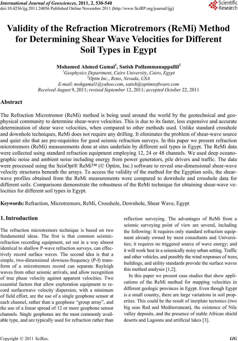International Journal of Geosciences, 2011, 2, 530-540
doi:10.4236/ijg.2011.24056 Published Online November 2011 (http://www.SciRP.org/journal/ijg)
Validity of the Refraction Microtremors (ReMi) Method
for Determining Shear Wave Velocities for Different
Soil Types in Egypt
Mohamed Ahmed Gamal1, Satish Pullammanappallil2
1Geophysics Department, Cairo University, Cairo, Egypt
2Optm Inc., Reno, Nevada, USA
Received August 9, 2011; revised September 12, 2011; accepted October 22, 2011
Abstract
The Refraction Microtremor (ReMi) method is being used around the world by the geotechnical and geo-
physical community to determine shear-wave velocities. This is due to its faster, less expensive and accura te
determination of shear wave velocities, when compared to other methods used. Unlike standard crosshole
and downhole techniques, ReMi does not require any drilling. It eliminates the problem of shear-wave source
and quiet site that are pre-requisites for good seismic refraction surveys. In this paper we present refraction
microtremors (ReMi) measurements done at sites underlain by different soil types in Egypt. The ReMi data
were collected using standard refraction equipment employing 12, 24 or 48 channels. We used deep oceano-
graphic noise and ambient noise including energy from power generators, pile drivers and traffic. The data
were processed using the SeisOpt® ReMi™ (© Optim, Inc.) software to reveal one-dimensional shear-wave
velocity structures beneath the arrays. To access the validity of the method for the Egyptian soils, the shear-
wave profiles obtained from the ReMi measurements were compared to downhole and crosshole data for
different soils. Comparisons demonstrate the robustness of the ReMi technique for obtaining shear-wave ve-
locities for different soil types in Egypt.
Keywords: Refraction, Microtremors, ReMi, Crosshole, Downhole, Shear Wave, Egypt
1. Introduction
The refraction microtremors technique is based on two
fundamental ideas. The first is that common seismic-
refraction recording equipment, set out in a way almost
identical to shallow P-wav e refraction surveys, can effec-
tively record surface waves. The second idea is that a
simple, two-dimensional slowness-frequency (P-f) trans-
form of a microtremors record can separate Rayleigh
waves from other seismic arrivals, and allow recognition
of true phase velocity against apparent velocities. Two
essential factors that allow exploration equipment to re-
cord surfacewave velocity dispersion, with a minimum
of field effort, are the use of a single geophone sensor at
each channel, rather than a geophone “group array”, and
the use of a linear spread of 12 or more ge ophone sensor
channels. Single geophones are the most commonly avail-
able type, and are typically used for refraction rather than
reflection surveying. The advantages of ReMi from a
seismic surveying point of view are several, including
the following: It requires only standard refraction equip-
ment already owned by most consultants and Universi-
ties; it requires no triggered source of wave energy; and
it will work best in a seismically noisy urban setting. Traffic
and other vehicles, and possibly the wind responses of trees,
buildings, and utility standards provide the surface waves
this method analyses [1,2].
In this paper we present case studies that show appli-
cations of the ReMi method for mapping velocities in
different geologic provinces in Egypt. Even though Egypt
is a small country, there are large variations in soil prop-
erties. This could be the result of inerplate tectonics (two
big seas Red and Mediterranean), the existence of Nile
valley deposits, and the presence of stable African shield
deserts and Lagoons and artificial lakes [3].

M. A. GAMAL ET AL.
531
2. Brief Geologic Setting of the Study Area
The study area is located in the northern part of Egypt.
The ReMi studies were conducted at eight sites located
between longitudes 29˚30' and 33˚E and latitudes 29˚ and
32˚N. The area is bound to the East by Gulf of Suez,
from north by the Mediterranean Sea Figure 1.
The River Nile plays a major role in the formation and
evolution of the alluvial deposits surrounding the Nile
Valley. The soil structure has evolved based on the in-
teraction between the Nile basin, Mediterranean Sea and
Gulf of Suez. Ground water exists at all sites except Mo-
kattam, which is located in a relatively high area.
Following is a b rief description of the geolog ic setting
of the eight sites [3].
2.1. Damietta
This area lies within the Mediterranean foreshore prov-
ince, an area of low relief terrain extending along the en-
tire northern coast Figure 1. The landforms are predomi-
nantly sand sheets and coastal depressions. Different b each
morphology is evident in the area. Changes in the sorting
processes have resulted in the following units:
1) River sand.
The Nile River sands are moderately sorted ranging in
size from fine-to medium-grained sands. This fluvial
facies is characterized by the presence of high percent-
ages of ooids, pyrite, sponge spicules and gypsum.
2) Coastal dune sand.
These are very well-sorted and are very rich in fine-to
medium grained laminated sands. They are characterized
by the lowest proportions of carbonate fragments and also
by the abundance of heavy minerals.
3) Accretion ridge sand.
This facies is very poorly sorted, varying in size from
very fine to coarse sands.
4) Beach sand.
The beach sands are well-sorted, fine to medium-
grained sands. This facies is characterized by presence of
heavy minerals as well as by the presence of some re-
worked marine biogenic components.
5) Near shore sand.
This facies is composed of poorly to moderately sorted
muddy sands. Carbonate fragments, ooids and gypsum are
relatively significant components.
6) Mud Facies.
This facies is composed of mixtures of silt and clay,
and have a low sand content.
7) Lagoon mud.
The lagoonal deposits have the highest proportions of
carbonate grains and nodules, plant remains, and shell
fragments.
Figure 1. Geologic map for northern Egypt showing the 8
ReMi test locations, 1-Damietta, 2-Sidi Krir, 3-Mahmoudia,
4-Nubaria, 5-EL Tebbin, 6-Alexandria, 7-Mokattam and 8-
Beni Suef [4].
2.2. Sidi Krir and Alexandria
Both these sites are located in the Mediterranean coastal
plain province. The Mediterranean coastal plain is charac-
terized by the presence of a number of elongated ridges
which run parallel to the coast, separated by longitudinal
depressions [3]. These ridges are composed mainly of
oolitic limestone. They seem to represent successive fossil
off-shore bars that were formed by the receding Mediterra-
nean during the Pleistocene. The depressions which separate
the bars contain lagoonal deposits (evaporites and marls).
2.3. Mahmoudia and Nubaria
Both of these sites lie within the Nile Valley and Nile
Delta deposits, where Wadi and playa deposits of quarter-
nary age are abundant Figure 1.
2.4. EL Tebbin
This site is characterized by Wadi deposits. They lie un-
conformably over the underlying Eocene limestone and
are made up of alternating poorly-bedded gravel beds
(sometimes reach thickness exceeding 20 m) and thin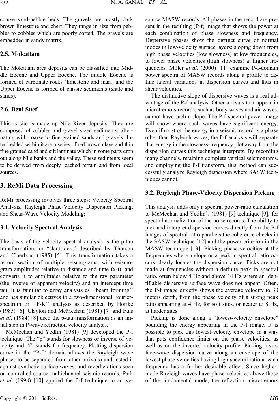

M. A. GAMAL ET AL.
532
coarse sand-pebble beds. The gravels are mostly dark
brown limestone and chert. They range in size from peb-
bles to cobbles which are poorly sorted. The gravels are
embedded in sandy matrix.
2.5. Mokattam
The Mokattam area deposits can be classified into Mid-
dle Eocene and Upper Eocene. The middle Eocene is
formed of carbonate rocks (limestone and marl) and the
Upper Eocene is formed of classic sediments (shale and
sands).
2.6. Beni Suef
This is site is made up Nile River deposits. They are
composed of cobbles and gravel sized sediments, alter-
nating with coarse to fine grained sands and gravels. In-
ter bedded within it are a series of red brown clays and thin
fine grained sand and silt laminate which in some parts crop
out along Nile banks and the valley. These sed iments seem
to be derived from deeply leached terrain and from local
sources.
3. ReMi Data Processing
ReMi processing involves three steps: Velocity Spectral
Analysis, Rayleigh Phase-Velocity Dispersion Picking,
and Shear-Wave Velocity Modeling:
3.1. Velocity Spectral Analysis
The basis of the velocity spectral analysis is the p-tau
transformation, or “slantstack,” described by Thorson
and Claerbout (1985) [5]. This transformation takes a
record section of multiple seismograms, with seismo-
gram amplitudes relative to distance and time (x-t), and
converts it to amplitudes relative to the ray parameter
(the inverse of apparent velocity) and an intercept time
tau. It is familiar to array analysts as ‘‘beam forming’’
and has similar objectives to a two-dimensional Fourier-
spectrum or ‘‘F-K’’ analysis as described by Horike
(1985) [6]. Clayton and McMechan (1981) [7] and Fuis
et al. (1984) [8] used the p-tau transformation as an ini-
tial step in P-wave refraction velocity analysis.
McMechan and Yedlin (1981) [9] developed the P-f
technique (The “p” stands for slowness or inverse of ve-
locity and “f” stands for frequency. Plotting dispersion
curve in the “P-f” domain allows the Rayleigh wave
phases to be separated from other arrivals) and tested it
against synthetic surface waves, and reverberations seen
on controlled-source multichannel seismic records. Park
et al. (1998) [10] applied the P-f technique to active-
source MASW records. All phases in the record are pre-
sent in the resulting (P-f) image that shows the power at
each combination of phase slowness and frequency.
Dispersive phases show the distinct curve of normal
modes in low-velocity surface layers: slop ing down from
high phase velocities (low slowness) at low frequencies,
to lower phase velocities (high slowness) at higher fre-
quencies. Miller et al. (2000) [11] examine P-f-domain
power spectra of MASW records along a profile to de-
fine lateral variations in dispersion curves and thus in
shear velocities.
The distinctive slope of dispersive waves is a real ad-
vantage of the P-f analysis. Other arrivals that appear in
microtremors records, such as body waves and air waves,
cannot have such a slope. The P-f spectral power image
will show where such waves have significant energy.
Even if most of the energy in a seismic record is a phase
other than Rayleigh wav es, the P-f analysis will separate
that energy in the slowness-frequency plot away from the
dispersion curves this technique interprets. By recording
many channels, retaining co mplete vertical seismogr ams,
and employing the P-f transform, this method can suc-
cessfully analyze Rayleigh dispersion where SASW tech-
niques cannot.
3.2. Rayleigh Phase-Velocity Dispersion Picking
This analysis adds only a spectral power-ratio calculation
to McMechan and Yedlin’s (1981) [9] technique [9], for
spectral normalization of the noise records. The ability to
pick and interpret dispersion curves d irectly from the P-f
images of spectral ratio parallels the coherence checks in
the SASW technique [12] and the power criterion in the
MASW technique [13]. Picking phase velocities at the
frequencies where a slope or a peak in spectral ratio oc-
curs clearly locates the dispersion curve. Picks are not
made at frequencies without a definite peak in spectral
ratio, often below 4 Hz and above 14 Hz where an iden-
tifiable dispersive surface wave does not appear. Often,
the P-f image directly shows the average velocity to 30
meters depth, from the phase velocity of a strong peak
ratio appearing at 4 Hz, for soft sites, or nearer to 8 Hz,
at harder sites.
Picking is done along a “lowest-velocity envelope”
bounding the energy appearing in the P-f image. It is
possible to pick this lowest-velocity envelope in a way
that puts confidence limits on the phase velocities, as
well as on the inverted velocity profile. Picking a sur-
face-wave dispersion curve along an envelope of the
lowest phase velocities having high spectral ratio at each
frequency has a further desirable effect. Since higher-
mode Rayleigh waves have phase velocities above those
of the fundamental mode, the refraction microtremors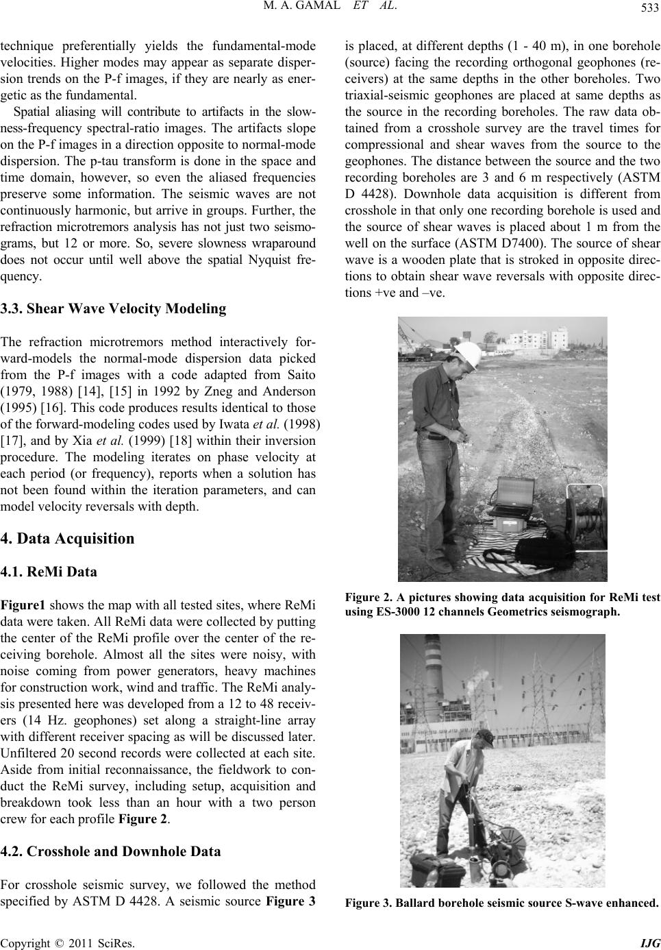

M. A. GAMAL ET AL.
533
technique preferentially yields the fundamental-mode
velocities. Higher modes may appear as separate disper-
sion trends on the P-f images, if they are nearly as ener-
getic as the fundamental.
Spatial aliasing will contribute to artifacts in the slow-
ness-frequency spectral-ratio images. The artifacts slope
on the P-f images in a direction opposite to normal-mode
dispersion. The p-tau transform is done in the space and
time domain, however, so even the aliased frequencies
preserve some information. The seismic waves are not
continuously harmonic, but arrive in groups. Further, the
refraction microtremors analysis has not just two seismo-
grams, but 12 or more. So, severe slowness wraparound
does not occur until well above the spatial Nyquist fre-
quency.
3.3. Shear Wave Velocity Modeling
The refraction microtremors method interactively for-
ward-models the normal-mode dispersion data picked
from the P-f images with a code adapted from Saito
(1979, 1988) [14], [15] in 1992 by Zneg and Anderson
(1995) [16]. This code produces results id entical to those
of the forward-modeling codes used by Iwata et al. (1998)
[17], and by Xia et al. (1999) [18] within their inversion
procedure. The modeling iterates on phase velocity at
each period (or frequency), reports when a solution has
not been found within the iteration parameters, and can
model velocity reversals with depth.
4. Data Acquisition
4.1. ReMi Data
Figure1 shows the map with all tested sites, where ReMi
data were taken. All ReMi data were collected by putting
the center of the ReMi profile over the center of the re-
ceiving borehole. Almost all the sites were noisy, with
noise coming from power generators, heavy machines
for construction work, wind and traffic. The ReMi analy-
sis presented here was developed from a 12 to 48 receiv-
ers (14 Hz. geophones) set along a straight-line array
with different receiver spacing as will be discussed later.
Unfiltered 20 second records were collected at each site.
Aside from initial reconnaissance, the fieldwork to con-
duct the ReMi survey, including setup, acquisition and
breakdown took less than an hour with a two person
crew for each profile Figure 2.
4.2. Crosshole and Downhole Data
For crosshole seismic survey, we followed the method
specified by ASTM D 4428. A seismic source Figure 3
is placed, at different depths (1 - 40 m), in one borehole
(source) facing the recording orthogonal geophones (re-
ceivers) at the same depths in the other boreholes. Two
triaxial-seismic geophones are placed at same depths as
the source in the recording boreholes. The raw data ob-
tained from a crosshole survey are the travel times for
compressional and shear waves from the source to the
geophones. The distance between the source and the two
recording boreholes are 3 and 6 m respectively (ASTM
D 4428). Downhole data acquisition is different from
crosshole in that only one recording borehole is used and
the source of shear waves is placed about 1 m from the
well on the surface (ASTM D7400). The source of shear
wave is a wooden plate that is stroked in opposite direc-
tions to obtain shear wave reversals with opposite direc-
tions +ve and –ve.
Figure 2. A pictures showing data acquisition for ReMi test
using ES-3000 12 channels Geometrics seismograph.
Figure 3. Ballard borehole seismic source S-wave enhanced.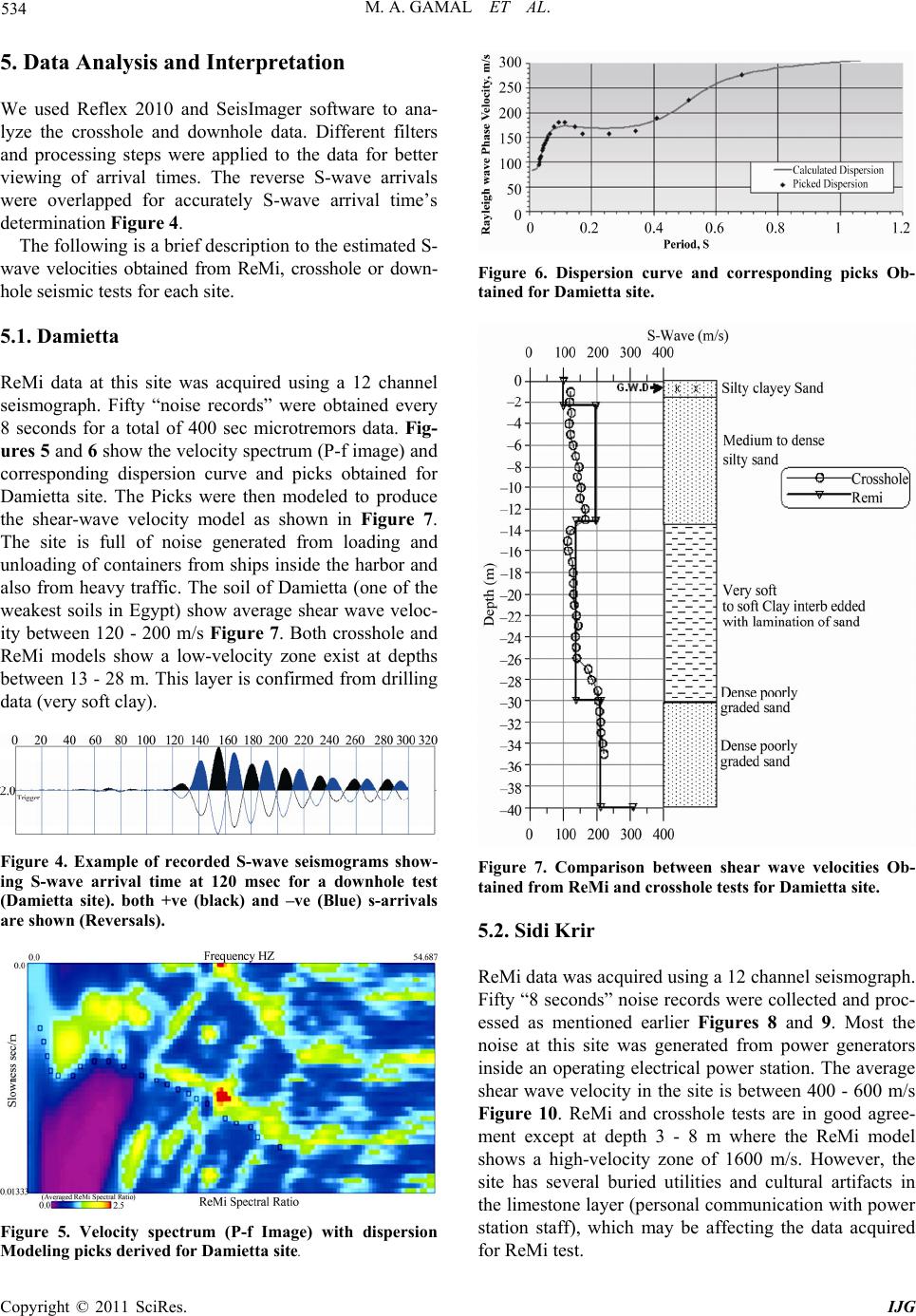

M. A. GAMAL ET AL.
534
5. Data Analysis and Interpretation
We used Reflex 2010 and SeisImager software to ana-
lyze the crosshole and downhole data. Different filters
and processing steps were applied to the data for better
viewing of arrival times. The reverse S-wave arrivals
were overlapped for accurately S-wave arrival time’s
determination Figure 4.
The following is a brief descriptio n to the estimated S-
wave velocities obtained from ReMi, crosshole or down-
hole seismic tests for each site.
5.1. Damietta
ReMi data at this site was acquired using a 12 channel
seismograph. Fifty “noise records” were obtained every
8 seconds for a total of 400 sec microtremors data. Fig-
ures 5 and 6 show the velocity spectrum (P-f image) and
corresponding dispersion curve and picks obtained for
Damietta site. The Picks were then modeled to produce
the shear-wave velocity model as shown in Figure 7.
The site is full of noise generated from loading and
unloading of containers from ships inside the harbor and
also from heavy traffic. The soil of Damietta (one of the
weakest soils in Egypt) show average shear wave veloc-
ity between 120 - 200 m/s Figure 7. Both crosshole and
ReMi models show a low-velocity zone exist at depths
between 13 - 28 m. This layer is confirmed from drilling
data (very soft clay).
Figure 4. Example of recorded S-wave seismograms show-
ing S-wave arrival time at 120 msec for a downhole test
(Damietta site). both +ve (black) and –ve (Blue) s-arrivals
are shown (Reversals).
Figure 5. Velocity spectrum (P-f Image) with dispersion
Modeling picks derived for Damietta site.
Figure 6. Dispersion curve and corresponding picks Ob-
tained for Damietta site.
Figure 7. Comparison between shear wave velocities Ob-
tained from ReMi and crosshole tests for Damietta site.
5.2. Sidi Krir
ReMi data was acquired using a 12 channel seismograph.
Fifty “8 seconds” noise records were collected and proc-
essed as mentioned earlier Figures 8 and 9. Most the
noise at this site was generated from power generators
inside an operating electrical power station. The average
shear wave velocity in the site is between 400 - 600 m/s
Figure 10. ReMi and crosshole tests are in good agree-
ment except at depth 3 - 8 m where the ReMi model
shows a high-velocity zone of 1600 m/s. However, the
site has several buried utilities and cultural artifacts in
the limestone layer (personal communication with power
station staff), which may be affecting the data acquired
for ReMi test.

M. A. GAMAL ET AL.
535
Figure 8. Velocity spectrum (P-f Image) with dispersion
Modeling picks derive d for Sidi Krir site .
Figure 9. Dispersion curve and corresponding picks Ob-
tained for Sidi Krir site.
Figure 10. Comparison between shear wave velocities Ob-
tained from ReMi And crosshole tests for Sidi Krir site.
5.3. Mahmoudia
ReMi data was acquired using a 12-channel system and
noise was dominated by loaders and hammers that were
demolishing old house at this site. This made acquiring
crosshole data a challenge at this site when compared
with ReMi data. Fifty records of noise “8 seconds each”
were collected. P-f image, Picks and corresponding dis-
persion curves are shown in Figures 11 and 12. The ob-
tained S-wave is between 100 - 350 m/s, ReMi data is
once again in good agreement with the crosshole data
Figure 13. The only big difference between ReMi and
crosshole data occur at depths between 30 - 40 m at
which crosshole source is not powerful enough to over-
come the noise in this site.
5.4. Nubaria
The soils underlying the Nubaria are very similar to that
of Mahmoudia (except the fill layer found at Mah-
moudia). Both are considered the extension to Nile delta
deposits. ReMi data acquisition was made using a 48
channel seismograph. Twenty records of “20 seconds”
each were collected resulting in a higher resolution P-f
images and dispersion curve Figures 14 and 15 com-
pared to the dispersion curves from 12 channel “8 sec-
ond” records. Figure 16 shows comparison of S-wave
Figure 11. Velocity spectrum (P-f Image) with dispersion
Modeling picks derived for Mahmoudia site.
Figure 12. Dispersion curve and corresponding picks Ob-
tained for Mahmoudia site.

M. A. GAMAL ET AL.
536
Figure 13. Comparison between shear wave velocities ob-
tained from ReMi and crosshole tests for Mahmoudia site.
Figure 14. Velocity spectrum (P-f Image) with dispersion
Modeling picks derived for Nubaria site.
Figure 15. Dispersion curve and corresponding picks ob-
tained for Nubaria site.
Figure 16. Comparison between shear wave velocities ob-
tained from ReMi and crosshole tests for Nubar ia site.
velocity obtained from ReMi models and crosshole or
downhole data. Using 48 channel 20 seconds make the
ReMi data in a better agreement to the crosshole data.
The obtained shear wave velocity is between 200 - 600
m/s. ReMi data succeeded at this site to show a shear
wave veloc i ty reversal for a dept h b etween 24 - 4 0 m.
5.5. EL Tebbin
The soils underlying the EL Tebbin site are very com-
plex due to the alternating layers of gravel sheets within
the soil column. Twenty files “20 seconds” each of ReMi
data were acquire d using a 48 ch ann el seismo grap h. D ata
collection was done at night, so the main noise u sed was
the deep oceanographic noise and little nearby traffic.
This was more than sufficient to generate a good disper-
sion curve Figures 17and 18. Figure 19 shows com-
parison between the models obtained from both ReMi,
and downhole data. The S-wave velocity is ranging be-
tween 300 - 1000 m/s.
5.6. Alexandria
Traffic and construction site activity provided ample
noise at this site. Twenty records “20 seconds” each were
collected using a 48 channel seismograph. P-f images

M. A. GAMAL ET AL.
537
and dispersion curves are shown in Figures 20 and 21.
The shear wave profile Figure 22 is ranging between
200 - 1400 m/s. No crosshole or downhole data were
collected for this site, however the S-wave velocity
model succeeds to monitor the bedrock depth at 13 m.
Figure 17. Velocity spectrum (P-f Image) with dispersion
Modeling picks derive d for EL Tebbin site.
Figure 18. Dispersion curve and corresponding picks ob-
tained for EL Tebbin site.
Figure 19. Comparison between shear wave velocities ob-
tained from ReMi and crosshole te sts for EL Tebbin site.
Figure 20. Velocity spectrum (P-f Image) with dispersion
Modeling picks derived for Alexanderia site.
Figure 21. Dispersion curve and corresponding picks ob-
tained for Alexanderia site.
Figure 22. Shear wave velocity obtained from ReMi test for
Alexanderia site.

M. A. GAMAL ET AL.
538
5.7. Mokattam
This site is underlain by limestone except for the upper
16 m which is composed of sand and sandstone. Twenty
files “20 seconds” each were collected for ReMi data
using a 48 channel seismograph. Deep noise and nearby
traffic provided ample noise at this site. The P-f image
and dispersion curves are shown in Figures 23 and 24.
The ReMi models Figure 25 show higher velocities at
17m that seem to correspond to the limestone bedrock.
5.8. Beni Suef
At this site the soil is rocky except in the upper 6 m
which is sandy gravel. No ReMi data were collected,
however shallow reflection survey data were acquired.
The reflection records were only 0.5 seconds long, re-
sulting in a low-resolution dispersion curve Figures 26
and 27 due to the shortness of the records. However the
curve was distinct and the picks made resulted in a
model that is in good agreement with the available
crosshole data. The average shear wave obtained is be-
tween 600-1200 m/s. The bedrock depth detected from
ReMi model is at about 9m depth Figure 28.
Figure 23. Velocity spectrum (P-f Image) with dispersion
Modeling picks derived for Mokattam site.
Figure 24. Dispersion curve and corresponding picks ob-
tained for Mokattam site.
Figure 25. Shear wave velocity obtained from ReMi test for
Mokattam site.
Figure 26. Velocity spectrum (P-f Image) with dispersion
Modeling picks deri ve d for Beni Suef site.
Figure 27. Dispersion curve and corresponding picks ob-
tained for Beni Suef site.

M. A. GAMAL ET AL.
539
Figure 28. Shear wave velocity obtained from ReMi Data,
using 0.5 seconds reflection records for Beni Suef site.
6. Conclusions
The limitations of ReMi are a result of the acquisition
parameters and frequency content of the noise being re-
corded. Maximum depth of resolution is the length of the
profile, with resolution decreasing with depth. The thin-
nest layer one can resolve is a function of geophone
spacing and maximum frequency of the recorded data.
Smaller geophone spacing and higher frequencies help
resolve thinner layers in the subsurface. Lower frequent-
cies provide resolution at depth. Ambient noise by itself
may lack high frequencies and so an active source (e.g.
hammer hits) can be used the augment the high fre-
quency content of the recorded data. We modeled the
dispersion picks by interactive forward modeling. We
started by using any number of layers and fit the disper-
sion picks by adding more layers, changing the velocity
of each layer and varying the depth of the layers. Mod-
eling was achieved by first starting with three layers and
fitting the high frequency dispersion picks that control
the shallow velocities. More layers were only added if
required by the data. Both velocities and depth of shal-
low layers are determined before the low frequency picks
are modeled to get velocities of the deeper layers.
The data were modeled blind without using constrains
from borehole or log d at a. However when compared both
data we found that the S-wave velocity given by ReMi
profiles like the abergae of the S-wave data given by
both crosshole or downhole data each time.
Eight different sites with different soils were investi-
gated to show the validity of ReMi Microtremors test In
Egypt, Damietta, Sidi Krir, Mahmoudia, Nubaria, EL
Tebbin, Alexanderia, Mokattam and Beni Suef. Almost
all soil types are sedimentary soil, varying between very
weak soil (soft clay at Damietta) into hard rock (Lime-
stone at Mokattam). At least 400 seconds microtremors
records were taken at each site using 48 channels or 12
channels Geometrics seismograph. Normal 14 Hz, geo-
phones were used in all tests. Almost all sites were found
very noisy from big machines such as electrical turbines
(power stations), construction activities (Loader and
hammers) or big winches for loading and unloading
(Damietta harbor).
Although some scientists are dealing with the longer
period microtremors originated from farther distances
(oceanographic disturbances) excluding urban excited
sites where high degree of local cultural noise ex ist [19],
we found that all previous kinds of noise are capable to
estimate good S-wave velocity models if compared with
other data (downhole and crosshole tests).
Our investigations have shown that the ReMi sur-
face-wave method is an excellent technique for deter-
mining the shear wave velocities. It compared very well
with crosshole and downhole results obtained from dif-
ferent soil types in Egypt. 20 seconds X 20 records (total
400 seconds) acquired using the 48 channel seismograph
gave high resolution P-f images and dispersion curves,
however 8 seconds X 50 records (total 400 seconds) us-
ing 12-channel records or 0.5 seconds X 200 records
(Total 100 seconds) reflection records also provided
good results – showing the robustness of the method. At
calm sites, P-f images were not good enough to estimate
good dispersion curves. In such a case it was better to
increase the amount of noise by driving a vehicle and
walking along the array or using hammer at the begin-
ning and end of the profile to generate surface waves.
Noisy sites provided the best data and these are the sites
were crosshole and downhole fail to give good signals. It
is better to collect ReMi data in these conditions. The
present study prov ed that the ReMi test is a very suitab le
test to be used in Egypt fo r different soils to estimate the
average shear wave velocity. Especially in very noisy
sites were crosshole sources will fail to overcome the
noise signals which is more powerful than the crosshole
source itself.
7. Acknowledgements
Sincere thanks to the all Electrical power stations staff

M. A. GAMAL ET AL.
540
who permitted the work kindly. Also Optim, who pro-
vided support and software.
8. References
[1] J. N. Louie, “Faster, Better: Shear-Wave Velocity to 100
Meters Depth from Refraction Microtremors Arrays,”
Bulletin of the Seismological Society of America, Vol. 91,
No. 2, 2001, pp. 347-364. doi:10.1785/0120000098
[2] S. Pullammanappallil, B. Honjas, J. Louie, J. A. Siemens
and H. Miura, “Comparative Study of the Refraction Mi-
crotremors Method: Using Seismic Noise and Standard
P-Wave Refraction Equipment for Deriving 1D Shear-
Wave Profiles,” Proceedings of the 6th SEGJ Interna-
tional Symposium, Tokyo, January 2003, pp. 192-197.
[3] R. Said, “The Geology of Egypt,” Conco Hurghada Inc.,
Rotterdam, 1990.
[4] EGSMA, Geological Map of Greater Cairo Area. Outline
of Geology Stratigraphy, Egyptian Geological Survey and
Mining Authority, 1983.
[5] J. R. Thorsonand J. F. Claerbout, “Velocity-Stack and
Slant-Stack Stochastic Inversion,” Geophysics, Vol. 50,
No. 12, 1985, pp. 2727-2741. doi:10.1190/1.1441893
[6] M. Horike, “Inversion of Phase Velocity of Long-Period
Microtremors to the S-Wave-Velocity Structure Down to
the Basement in Urbanized Areas,” Journal of Physics of
the Earth, Vol. 33, 1985, pp. 59-96.
doi:10.4294/jpe1952.33.59
[7] R. W. Clayton and G. A. McMechan, “Inversion of Re-
fraction Data by Wavefield Continuation,” Geophysics,
Vol. 46, No. 3, 1981, pp. 860-868.
doi:10.1190/1.1441224
[8] G. Fuis, W. Mooney, J. Healy, G. McMechan and W.
Lutter, “A Seismic Refraction Survey of the Imperial
Valley Region, California,” Journal of Geophysical Re-
search, Vol. 89, No. B2, 1984, pp. 1165-1190.
doi:10.1029/JB089iB02p01165
[9] G. A. McMechan and M. J. Yedlin, “Analysis of Disper-
sive Waves by Wave Field Transformation,” Geophysics,
Vol. 46, No. 6, 1981, pp. 869-874.
doi:10.1190/1.1441225
[10] C. B. Park, R. D. Miller and J. Xia, “Imaging Dispersion
Curves of Surface Waves on Multi-Channel Record,”
Annual Meeting Abstracts, Society of Exploration Geo-
physicists, Tulsa, 1998, pp. 1377-1380.
[11] R. D. Miller, C. B. Park, J. M. Ivanov, J. Xia, D. R. Laf-
len, and C. Gratton, “MASW to Investigate Anomalous
Near-Surface Materials at the Indian Refinery in Law-
renceville,” Kansas Geology Survey, Open-File Report,
Lawrence,2000, p. 48.
[12] S. Nazarian and K. H. Stokoe II, “In Situ Shear Wave
Velocities from Spectral Analysis of Surface Waves,”
Proceedings of the World Conference on Earthquake En-
gineering, Vol. 8, San Francisco, 21-28 July 1984.
[13] C. B. Park, R. D. Miller and J. Xia, “Multi-Channel
Analysis of Surface Waves,” Geophysics, Vol. 64, No. 3,
1999, pp . 8 0 0 - 8 0 8 . doi:10.1190/1.1444590
[14] M. Saito, “Computations of Reflectivity and Surface
Wave dispersion Curves for Layered Media; I, Sound
Wave and SH Wave,” Butsuri-Tanko, Vol. 32, No. 5,
1979, pp. 15-26.
[15] M. Saito, “Compound Matrix Method for the Calculation
of Spheroidal Oscillation of the Earth,” Seismological
Research Letters, Vol. 59, 1988, p. 29.
[16] Y. Zeng and J. G. Anderson, “A Method for Direct Com-
putation of the Differential Seismograms with Respect to
the Velocity Change in a Layered Elastic Solid,” Bulletin
of the Seismological Society of America, Vol. 85, No. 1,
1995, pp. 300-307.
[17] T. Iwata, H. Kawase, T. Satoh, Y. Kakehi, K. Irikura, J.
N. Louie, R. E. Abbott and J. G. Anderson, “Array Mi-
crotremor Measurements at Reno, Nevada, USA,” EOS,
Transactions of the American Geophysical Union, Vol.
79, No. 45, p. F578.
[18] J. Xia, R. D. Miller and C. B. Park, “Estimation of
Near-Surface Shear-Wave Velocity by Inversion of Ray-
leigh Wave,” Geophysics, Vol. 64, No. 3, 1999, pp. 691-
700. doi:10.1190/1.1444578
[19] E. H. Field, S. E. Hough and H. Jacob, “Using Mi-
crotremors to Assess Potential Arthquake Site Response,
a Case Study in Flushing Meadows, New York City,”
Bulletin of the Seismological Society of America, Vol. 80,
No. 6A, 1990, pp. 1456-1480.