Spatial analysis of tuberculosis in four main ethnic communities in Taiwan during 2005 to 2009

doi:10.4236/ojpm.2011.13017

Paper Menu >>

Journal Menu >>

Vol.1, No.3, 125-134 (2011)

doi:10.4236/ojpm.2011.13017

Open Journal of Preventive Medicine

Spatial analysis of tuberculosis in four main ethnic

communities in Taiwan during 2005 to 2009

Pui-Jen Tsai

Center for General Education, Aletheia University, New Taipei, Taiwan; puijentsai@gmail.com

Received 5 September 2011; revised 16 October 2011; accepted 25 October 2011.

ABSTRACT

The aim of the pres e nt s tu dy was to assess sp a -

tial features of tuberculosis prevalence and

their relationships with four main ethnic com-

munities in Taiwan. Methods of spatial analysis

were clustering pattern determination (such as

global version of Moran’s test and local version

of Gi*(d) statistic), using logistic regression cal-

culations to identify spatial distributions over a

contiguous five years and identify significant

similarities, discriminant analysis to classify va-

riables, and geographically weighted regression

(GWR) to determine the strength of relation-

ships between tuberculosis prevalence and eth-

nic variables in spatial features. Tuberculosis

demonstrated decreasing trends in prevalence

in both genders during 2005 to 2009. All results

of the global Moran’s tests indicated spatial he-

terogeneity and clusters in the plain and moun-

tainous Aboriginal townships. The Gi*(d) statis-

tic calculated z-score outcomes, categorized as

clusters or non-clusters, at at 5% significance

level. According to the stepwise Wilks’ lambda

discriminant analysis, in the Aborigines and

Hoklo communities townships with clusters of

tuberculosis cases differentiated from town-

ships without cluster cases, to a greater extent

than in the other communities. In the GWR mo-

dels, the explanatory variables demonstrated

significant and positive signs of parameter es-

timates in clusters occurring in plain and moun-

tainous aboriginal townships. The explanatory

variables of both the Hoklo and Hakka commu-

nities demonstrated significant, but negative,

signs of parameter estimates. The Mainlander

community did not significantly associate with

cluster patterns of tuberculosis in Taiwan. Re-

sults indicated that locations of high tuberculo-

sis prevalence closely related to areas contain-

ing higher proportions of the Aboriginal c o mm u -

nity in Taiwan. This information is relevant for

assessment of spatial risk factors, which, in

turn, can facilitate the planning of the most ad-

vantageous types of health care policies, and

im pl e m en t a ti o n of ef f e ct i ve h e al t h ca r e s e rv ices.

Keywords: Tuberculosis; Taiwane se Ethnicity;

Global Moran’s Test; Local Gi*(d) Statistic; Logistic

Regression; Discrimin ant Analysis; Geographic a lly

Weighted Regression

1. INTRODUCTION

Tuberculosis (TB) is one of the world’s principal in-

fectious diseases. In 2007, the World Health Organiza-

tion (WHO) estimated that more than nine million new

cases of TB occur globally, with more than half of these

new cases occurring in Asia (55%). Approximately 1.76

million people died of TB worldwide in 2007. In recent

years, with increasing numbers of cases of human im-

munodeficiency virus (HIV) and multidrug resistant

tuberculosis (MDR-TB), prevention of TB has posed a

significant challenge. TB is an infectious disease, caused

by mycobacteria of the M. tuberculosis complex (M.

tuberculosis, M. bovis, M. africanum, M. microti, M. ca-

nettii, M. caprae, M. pinnipedii). Transmission occurs

via exposure to tubercle bacilli in airborne droplet nuclei

produced by a person with infectious TB during cough-

ing, sneezing, singing, or talking. The infectiousness of

the person with TB, the susceptibility of those exposed,

the duration of exposure, the proximity to the source

case, and the efficiency of cabin ventilation are all fac-

tors which can influence the risk of infection. Suscepti-

bility to infection and disease increases in immunocom-

promised persons (such as human immunodeficiency

virus-infected persons) and infants and young children

(less than five years of age). When TB develops in the

human body, it does so in two stages: first, the individual

exposed to M. tuberculosis becomes infected, and sec-

ond, the infected individual develops the disease (active

TB). A small minority (<10%) of infected individuals

P.-J. Tsai / Open Journal of Preventive Medicine 1 (2011) 125-134

126

subsequently develop active disease and most of them do

so within five years. The risk of progression to active TB

disease is greatest within the first two years after infec-

tion. However, latent infection may persist for life [1,2].

Taiwan has engaged in TB prevention for more than

50 years. For nearly a decade, both the incidence and

death rates of TB in Taiwan have gradually declined, yet

it remains a prominent infectious disease with the largest

number of annual confirmed cases and deaths among all

notifiable infectious diseases. According to the Taiwan

Tuberculosis Control Report (2009), during each year

from to 2005 to 2008 the tuberculosis incidence was

16,472 (72.5 per 100,000 population), 15,378 (67.4 per

100,000 population), 14,480 (63.2 per 100,000 popula-

tion), and 14,265 (62.0 per population), respectively.

Overall, the incidence decreased by 14.5%. The inci-

dence rates of all forms of TB and smear-positive TB in

males were two to three times higher than in females in

2007. Irrespective of gender, incidence rates increased

with age. The numbers of deaths caused by TB cause

during each year from 2005 to 2008 were 970 (4.3 per

100,000 population), 832 (3.6 per 100,000 population),

783 (3.4 per 100,000 population), and 762 (3.3 per

100,000 population), respectively. Overall, mortalities

decreased by 23.3%.However, the decline in the number

of new TB cases in Taiwan was less significant than

declines occurring in the U.S., Japan, and Singapore [2].

In a 12 month cohort study in 2006 the treatment suc-

cess rate of all forms of new TB cases was 70.4%, and

the death rate was 18.6%. Of all regions, Central Tai-

wan had the highest treatment success rate (72.8%),

while the Eastern area had the lowest (63.0%). Accord-

ing to the number of smear-positive TB cases in 2006

and the treatment outcomes of 12 months cohort study,

the 2009 WHO Tuberculosis Annual Report described

the global success rate as 84.3% (for the 2006 cohort),

achieving the Millennium Development Goal (MDG) of

85% designated by the WHO. In Taiwan, the treatment

success rate of smear-positive cases in a 12 month co-

hort study was 67%. This value was higher than the rates

observed in Japan (53%) and the U.S. (64%), but lower

than in Singapore (84%), and did not achieve the WHO

assigned target [2].

A number of reports have documented that habitation

in mountain aboriginal townships and age of 65 years

are two factors which closely associate with the inci-

dence and prevalence of tuberculosis in Taiwan [3-7].

However, research on healthcare problems associated

with tuberculosis in Taiwanese ethnic people is limited.

The present study employs methods of spatial analysis of

areal data to determine spatial features related to tuber-

culosis and the four major Taiwanese communities.

2. METHODS

2.1. Study Area

The study was conducted within the main island of

Taiwan (excluding all islets), which, in 2008, comprised

more than 23 million inhabitants living in an area of

36,000 km2. A total of 349 local administrative govern-

ment areas, including five main urban areas, two second-

dary urban areas, 162 rural townships, and 54 plain and

mountainous aboriginal townships, were assessed (Fig-

ure 1). According to a bulletin from the Ministry of In-

terior, issued in 2002, urban areas are regions having at

least one metropolitan centre and can include neigh-

bouring cities and townships which share socioeconomic

activities. Main urban areas are defined as those with a

population larger than one million; specifically, Taipei-

Keelung, Kaohsiung, Taichung-Changhua, JhongliTao-

yuan, and Tainan. Secondary urban areas are defined as

those with a residential population ranging from 0.3 to 1

million (Hsinchu and Chiayi) [8].

2.2. Data Collection and Management

The Taiwan National Health Insurance (NHI) program

was initiated in 1995. The coverage rate of the program

increased from 92.41% in 1995 to more than 96.16% in

2000, and then further increased to 98% after the inclu-

sion of active military forces in 2001. At the beginning

of 2004, NHI data related to medical care, such as the

leading causes of death, were reclassified and reproc-

essed in relation to smaller units or areas (for example,

precincts or townships rather than the country as a

Figure 1. Map of urban regions and aboriginal townships in

the study area. Map of the study area divided into 349 admin-

istrative districts including 7 urban regions and an integrated

area of 54 plain and mountainous aboriginal townships.

P.-J. Tsai / Open Journal of Preventive Medicine 1 (2011) 125-134

127

whole). Regional data from the statistical analysis sys-

tem (SAS) program are announced publicly by the NHI

in regular annual reports (for example, NHI, 2005-2009).

These reports provide an accurate and reliable data

source to researchers for investigation of health care

issues in Taiwan [9-13]. The data were collected from

contractual medical care institutions, which, in the pre-

sent study, are institutions where the NHI covers pre-

scription medicinal costs and treatment at outpatient

clinics. Such facilities accumulate detailed databases of

medical costs for inpatient care. The numbers of outpa-

tient cases were classified in relation to disease codes, as

defined in the 1975 edition of “The International Classi-

fication of Diseases, 9th Revision, Clinical Modifica-

tion” (hereafter, ICD 9 CM), 2005-2007 and “The Tenth

Revision of the International Statistical Classification of

Diseases and Related Health Problems” (hereafter, ICD

10 CM), 2008-2009. Criteria for refining the data were

first established. However, for calculating medical costs

and numbers of visits, the disease code of the first group

(main diagnosis code) was used as the cause of disease.

Selected data were not included in the final statistical

data set, such as cases where patients suffered from dis-

eases which defied code classification, or had mis-

matched ID numbers. Disease codes were classified ac-

cording to gender and age. Cases sharing the same ID

numbers, despite having different diseases, were counted

as separate incidences.

Medical care data obtained from the NHI, 2005-2009

reports were examined, and the prevalence rates of tu-

berculosis (ICD 02, according to ICD 9 CM standards in

2005-2007 and the disease code of tuberculosis A15-

A19, classified by ICD 10 CM in 2008-2009) were cal-

culated. The Ministry of the Interior provided the demo-

graphic information (the mid-year population of each

township) [8]. The age-adjusted standard prevalence

rates were calculated with a direct adjustment using the

world population in 2000 as the standard population [14].

The age-adjusted standard prevalence rates during 2005-

2009 were calculated according to which of the five year

prevalence rates were weighted by persons each year and

(or) by persons each gender. The results provided tuber-

culosis prevalence rates for males and females in the

whole of Taiwan and in each township in the study area,

and these were consequently applied to spatial autocor-

relation analysis.

The percentages of the four major Taiwanese ethnic

communities in each township were obtained from an

official report of the Council for Hakka Affairs (2004)

[15]. According to self-reports in official governmental

statistics, Han Chinese constitute 98% of Taiwan’s po-

pulation, while Taiwanese Aborigines constitute the re-

maining 2%. The composite category of “Taiwanese

people” is often reputed to include a significant popula-

tion of at least four constituent ethnic groups: the Hoklo

(73.3%), the Hakka (13.5%), the Mainlander (8%), and

the Taiwanese Aborigines (1.9%) [15]. Figure 2 maps

the proportions of ethnic communities in populations of

each of the 349 townships.

2.3. Global Moran’s I Statistic

The global spatial autocorrelation statistical method

was used to evaluate correlation between neighbouring

observations, and to identify patterns and levels of spa-

tial clustering in neighbouring districts [16]. The Moran’s

I statistic, similar to the Pearson correlation coefficient

[17], is calculated using:



ux u

Sxu





  (1)

where N is the number of districts and wij is the element

in the spatial weight matrix corresponding to the obser-

vation pair i, j. xi and xj are observations for areas i and j

(a) (b)

Figure 2. Maps of population percentages of four Taiwanese

ethnic communities in the study area. (a) Hoklo community. (b)

Hakka community. (c) Mainlander community. (d) Aboriginal

community.

P.-J. Tsai / Open Journal of Preventive Medicine 1 (2011) 125-134

128

with mean u and

S (2)

Since the weights are row-standardized and 1





the first step in the spatial autocorrelation analysis was

to construct a spatial weight matrix which contained

information about the neighbourhood structure for each

location. Adjacency was defined as immediately neigh-

boring administrative districts, inclusive of the district

itself. Non-neighbouring administrative districts were

assigned a weight of zero.

Spatial contiguity for polygons is the property of

sharing a common boundary or vertex. Contiguity analy-

sis is an important method for assessing unusual features

in the connectivity distribution [18,19]. The Queen’s

measure of contiguity can be utilized to make up for

spatial contiguity by incorporating both the Rook and

Bishop relationships into a single measure [19].

The administrative districts considered in this study

were highly irregular in both shape and size. Tsai et al.

(2009) demonstrated that the most appropriate method

for quantifying the spatial weights matrix for analysis of

connectivity is the first order queen polygon continuity

method [7]. The spatial weights/connectivity matrices

were utilized in local Gi*(d) calculations.

2.4. Local Gi*(d) Statistic

The local Gi*(d) statistic (local G-statistic) is used to

determine the statistical significance of local clusters,

and to evaluate the spatial extent of these clusters

[20,21]. The local G-statistic is useful for identifying

individual members of local clusters by determining the

spatial dependence and relative magnitudes between an

observation and neighboring observations [22]. The lo-

cal G-statistic can be written as follows [20,23,24]:



()

(), for all

jijj i

wdx Wx

Gd j

nS W







 (3)

where x is a measure of the prevalence rate of tuberculo-

sis within a given polygon (each administrative district),

wij is a spatial weight which defines neighbouring ad-

ministrative districts j to i, Wi is the sum of the weights

wij, 1j

, ,

1ii

Swj

1jj



.

Developing the spatial weight wij is the first step to

calculating Gi*(d). The spatial weight matrix includes wij

= 1. In the present study, adjacency was defined using a

first order queen polygon continuity weight file which

had been constructed based on the districts which share

common boundaries and vertices.

Non-neighbouring administrative districts were as-

signed a weight of zero. The neighbours of an adminis-

trative district were defined as those with which the ad-

ministrative district shares a boundary. This formed a

simple 0/1 matrix; 1 indicated that the municipalities

share a common border or vertex, 0 otherwise [23,25].

The local G-statistic included the value in the calcula-

tion at i. Assuming that G

i*(d) is approximately nor-

mally distributed [20], the output of Gi*(d) can be cal-

culated as a standard normal variant with an associated

probability from the z-score distribution [26]. Clusters

with a 95% significance level from a two-tailed normal

distribution indicated significant spatial clustering, but

only positively significant clusters (z-score values grea-

ter than +1.96) were mapped.

2.5. To Determine Space-Time Similarities

Using Logistic Regression Model

Similarities between spatial distribution patterns for a

time course during 2005 to 2009 were determined using

logistic regression model. The binary response indicated

if there was significant autocorrelation between admin-

istrative districts or areas. If the absolute value of the

z-score of the local G-statistics was larger than 1.96 this

indicated higher correlation; lower correlation if other-

wise. Year was considered an explanatory variable in the

logistic regression model. Thus, the model could be ex-

pressed as:







PrHigher correlation

log PrLower correlationYear











(4)

where 0



and 1



are the logistic regression coeffi-

cients of the model. Pr (Higher correlation) and Pr

(Lower correlation) denote the “Higher” and “Lower”

correlation probabilities, respectively.

2.6. Discriminant Analysis

Discriminant analysis is useful for determining which

variables discriminate between two or more groups,

building a predictive model of group membership based

on observed characteristics of each case [27]. It provides

a multiple regression equation(s) and those variables

which contribute most to the discrimination of group

membership are the ones with the largest standardized

coefficients. Discrimination analysis is less flexible than

regression because it requires the explanatory variables

to be normally distributed without equal variance within

each group [28]. Using the discriminant analysis, Tai-

wanese ethnic variables could be identified in the study

area. A stepwise Wilks’ lamda discriminant analysis was

applied to compare tuberculosis prevalence (2005 to

2009) within the townships of Gi*(d) test’s clusters to

those classified as non-clustered relative to four Tai-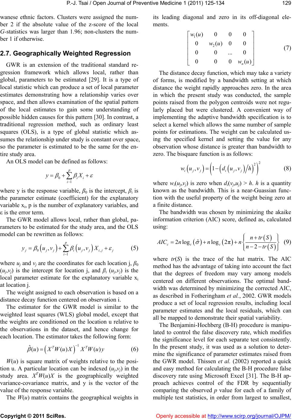

P.-J. Tsai / Open Journal of Preventive Medicine 1 (2011) 125-134

129

wanese ethnic factors. Clusters were assigned the num-

ber 2 if the absolute value of the z-score of the local

G-statistics was larger than 1.96; non-clusters the num-

ber 1 if otherwise.

2.7. Geographically Weighted Regression

GWR is an extension of the traditional standard re-

gression framework which allows local, rather than

global, parameters to be estimated [29]. It is a type of

local statistic which can produce a set of local parameter

estimates demonstrating how a relationship varies over

space, and then allows examination of the spatial pattern

of the local estimates to gain some understanding of

possible hidden causes for this pattern [30]. In contrast, a

traditional regression method, such as ordinary least

squares (OLS), is a type of global statistic which as-

sumes the relationship under study is constant over space,

so the parameter is estimated to be the same for the en-

tire study area.

An OLS model can be defined as follows:







 



where y is the response variable, β0 is the intercept, βi is

the parameter estimate (coefficient) for the explanatory

variable xi, p is the number of explanatory variables, and

ε is the error term.

The GWR model allows local, rather than global, pa-

rameters to be estimated for the study area, and the OLS

model can be rewritten as follows:

 

jji jjijj

yuv uvX











)

(5)

where uj and vj are the coordinates for each location j, β0

(uj,vj) is the intercept for location j, and βi (uj,vj) is the

local parameter estimate for the explanatory variable xi

at location j.

The weight assigned to each observation is based on a

distance decay function centered on observation i.

The estimator for the GWR model is similar to the

weighted least squares (WLS) global model, except that

the weights are conditioned on the location u relative to

the observations in the dataset, and hence change for

each location. The estimator takes the following form:



ˆ() ()()

uXWuXXWu





 (6)

W(u) is square matrix of weights relative to the posi-

tion u. A particular location can be indexed (uj,vj) in the

study area. XTW(u)X is the geographically weighted

variance-covariance matrix, and y is the vector of the

value of the response variable.

The W(u) matrix contains the geographical weights in

its leading diagonal and zero in its off-diagonal ele-

ments.

() 000

0()00

00...0

000(

























(7)

The distance decay function, which may take a variety

of forms, is modified by a bandwidth setting at which

distance the weight rapidly approaches zero. In the area

in which the present study was conducted, the sample

points raised from the polygon centroids were not regu-

larly placed but were clustered. A convenient way of

implementing the adaptive bandwidth specification is to

select a kernel which allows the same number of sample

points for estimations. The weight can be calculated us-

ing the specified kernel and setting the value for any

observation whose distance is greater than bandwidth to

zero. The bisquare function is as follows:

 







,1 ,

ijj ijj

wuvduv h (8)

where wi(uj,vj) is zero when di(vj,uj) > h. h is a quantity

known as the bandwidth. This is a near-Guassian func-

tion with the useful property of the weight being zero at

a finite distance.

The bandwidth was chosen by minimizing the akaike

information criterion (AIC) score, defined as, calculated

using:

 







2loglog 2π

cc c

ntrS

AICnnn ntrS



















(9)

where tr(S) is the trace of the hat matrix. The AIC

method has the advantage of taking into account the fact

that the degrees of freedom may vary among models

centered on different observations. The optimal band-

width was determined by minimizing the corrected AIC,

as described in Fotheringham et al., 2002. GWR models

produce a set of local regression results, including local

parameter estimates and the local residuals, which can

all be mapped to demonstrate their spatial variability.

The Benjamini-Hochberg (B-H) procedure is manipu-

lated to control the false discovery rate, which modifies

the significance level for each separate test consistently.

In the present study, it was used as a solution to deter-

mine the significance of parameter estimates raised from

the GWR model. Thissen et al. (2002) reported a quick

and easy method for calculating the B-H procedure false

discovery rate using Microsoft Excel [31]. The B-H ap-

proach achieves control of the FDR by sequentially

comparing the observed p value for each of a family of

multiple test statistics, in order from largest to smallest,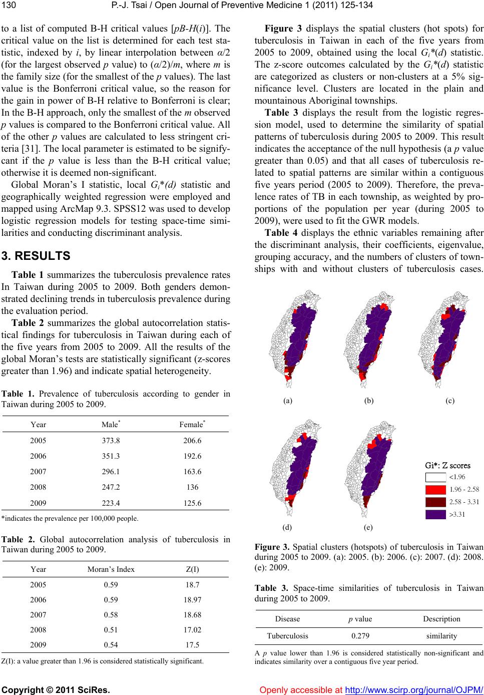

P.-J. Tsai / Open Journal of Preventive Medicine 1 (2011) 125-134

130

to a list of computed B-H critical values [pB-H(i)]. The

critical value on the list is determined for each test sta-

tistic, indexed by i, by linear interpolation between α/2

(for the largest observed p value) to (α/2)/m, where m is

the family size (for the smallest of the p values). The last

value is the Bonferroni critical value, so the reason for

the gain in power of B-H relative to Bonferroni is clear;

In the B-H approach, only the smallest of the m observed

p values is compared to the Bonferroni critical value. All

of the other p values are calculated to less stringent cri-

teria [31]. The local parameter is estimated to be signify-

cant if the p value is less than the B-H critical value;

otherwise it is deemed non-significant.

Global Moran’s I statistic, local Gi*(d) statistic and

geographically weighted regression were employed and

mapped using ArcMap 9.3. SPSS12 was used to develop

logistic regression models for testing space-time simi-

larities and conducting discriminant analysis.

3. RESULTS

Table 1 summarizes the tuberculosis prevalence rates

In Taiwan during 2005 to 2009. Both genders demon-

strated declining trends in tuberculosis prevalence during

the evaluation period.

Table 2 summarizes the global autocorrelation statis-

tical findings for tuberculosis in Taiwan during each of

the five years from 2005 to 2009. All the results of the

global Moran’s tests are statistically significant (z-scores

greater than 1.96) and indicate spatial heterogeneity.

Table 1. Prevalence of tuberculosis according to gender in

Taiwan during 2005 to 2009.

Year Male* Female*

2005 373.8 206.6

2006 351.3 192.6

2007 296.1 163.6

2008 247.2 136

2009 223.4 125.6

*indicates the prevalence per 100,000 people.

Table 2. Global autocorrelation analysis of tuberculosis in

Taiwan during 2005 to 2009.

Year Moran’s Index Z(I)

2005 0.59 18.7

2006 0.59 18.97

2007 0.58 18.68

2008 0.51 17.02

2009 0.54 17.5

Z(I): a value greater than 1.96 is considered statistically significant.

Figure 3 displays the spatial clusters (hot spots) for

tuberculosis in Taiwan in each of the five years from

2005 to 2009, obtained using the local Gi*(d) statistic.

The z-score outcomes calculated by the Gi*(d) statistic

are categorized as clusters or non-clusters at a 5% sig-

nificance level. Clusters are located in the plain and

mountainous Aboriginal townships.

Table 3 displays the result from the logistic regres-

sion model, used to determine the similarity of spatial

patterns of tuberculosis during 2005 to 2009. This result

indicates the acceptance of the null hypothesis (a p value

greater than 0.05) and that all cases of tuberculosis re-

lated to spatial patterns are similar within a contiguous

five years period (2005 to 2009). Therefore, the preva-

lence rates of TB in each township, as weighted by pro-

portions of the population per year (during 2005 to

2009), were used to fit the GWR models.

Table 4 displays the ethnic variables remaining after

the discriminant analysis, their coefficients, eigenvalue,

grouping accuracy, and the numbers of clusters of town-

ships with and without clusters of tuberculosis cases.

(a) (b) (c)

Gi*: Z scores

<1.96

1.96 - 2.58

2.58 - 3.31

>3.31

(d) (e)

Figure 3. Spatial clusters (hotspots) of tuberculosis in Taiwan

during 2005 to 2009. (a): 2005. (b): 2006. (c): 2007. (d): 2008.

(e): 2009.

Table 3. Space-time similarities of tuberculosis in Taiwan

during 2005 to 2009.

Disease p value Description

Tuberculosis 0.279 similarity

A p value lower than 1.96 is considered statistically non-significant and

indicates similarity over a contiguous five year period.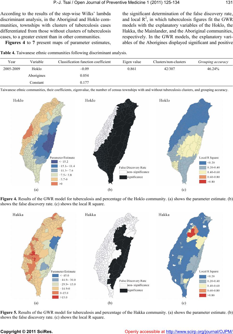

P.-J. Tsai / Open Journal of Preventive Medicine 1 (2011) 125-134

131

According to the results of the step-wise Wilks’ lambda

discriminant analysis, in the Aboriginal and Hoklo com-

munities, townships with clusters of tuberculosis cases

differentiated from those without clusters of tuberculosis

cases, to a greater extent than in other communities.

Figures 4 to 7 present maps of parameter estimates,

the significant determination of the false discovery rate,

and local R2, in which tuberculosis figures fit the GWR

models with the explanatory variables of the Hoklo, the

Hakka, the Mainlander, and the Aboriginal communities,

respectively. In the GWR models, the explanatory vari-

ables of the Aborigines displayed significant and positive

Table 4. Taiwanese ethnic communities following discriminant analysis.

Year Variable Classification function coefficient Eigen value Clusters/non-clusters Grouping accuracy

2005-2009 Hoklo –0.09 0.861 42/307 46.24%

Aborigines 0.054

Constant 0.177

Taiwanese ethnic communities, their coefficients, eigenvalue, the number of census townships with and without tuberculosis clusters, and grouping accuracy.

(a) (b) (c)

Figure 4. Results of the GWR model for tuberculosis and percentage of the Hoklo community. (a) shows the parameter estimate. (b)

shows the false discovery rate. (c) shows the local R square.

(a) (b) (c)

Figure 5. Results of the GWR model for tuberculosis and percentage of the Hakka community. (a) shows the parameter estimate. (b)

shows the false discovery rate. (c) shows the local R square.

Openly accessible at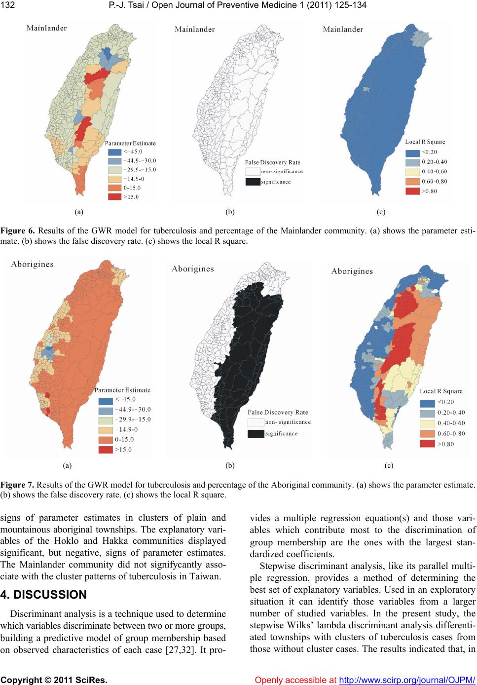

P.-J. Tsai / Open Journal of Preventive Medicine 1 (2011) 125-134

132

(a) (b) (c)

Figure 6. Results of the GWR model for tuberculosis and percentage of the Mainlander community. (a) shows the parameter esti-

mate. (b) shows the false discovery rate. (c) shows the local R square.

(a) (b) (c)

Figure 7. Results of the GWR model for tuberculosis and percentage of the Aboriginal community. (a) shows the parameter estimate.

(b) shows the false discovery rate. (c) shows the local R square.

signs of parameter estimates in clusters of plain and

mountainous aboriginal townships. The explanatory vari-

ables of the Hoklo and Hakka communities displayed

significant, but negative, signs of parameter estimates.

The Mainlander community did not signifycantly asso-

ciate with the cluster patterns of tuberculosis in Taiwan.

4. DISCUSSION

Discriminant analysis is a technique used to determine

which variables discriminate between two or more groups,

building a predictive model of group membership based

on observed characteristics of each case [27,32]. It pro-

vides a multiple regression equation(s) and those vari-

ables which contribute most to the discrimination of

group membership are the ones with the largest stan-

dardized coefficients.

Stepwise discriminant analysis, like its parallel multi-

ple regression, provides a method of determining the

best set of explanatory variables. Used in an exploratory

situation it can identify those variables from a larger

number of studied variables. In the present study, the

stepwise Wilks’ lambda discriminant analysis differenti-

ated townships with clusters of tuberculosis cases from

those without cluster cases. The results indicated that, in

P.-J. Tsai / Open Journal of Preventive Medicine 1 (2011) 125-134

133

the Aboriginal and Hoklo communities, townships with

clusters of tuberculosis cases differentiated from those

without cluster cases to a greater extent than in other

communities. However, this analysis could only provide

the best set of explanatory variables in global version.

GWR is a local version of spatial regression which

generates parameters disaggregated by the spatial units

of analysis. This allows the assessment of spatial

heterogeneity in the estimated relationships between the

response and explanatory variables. In the global model,

it is usual to test whether the parameter (referred to as

the coefficient) estimates significantly differ from zero.

This can be accomplished with a t-test, in which the

output provides the t statistics and their associated p

values. A parameter may have a value estimated as little

more than zero; therefore associated with a variable

whose variation does not contribute to the model. The

model excludes variables with non-significant parameter

estimates. In the GWR, one set of parameters associates

with each regression point, as well as one set of standard

errors, therefore potentially hundreds or thousands of

tests would be required to determine if parameters are

locally significant. Parameter estimates for variables

close to zero often have a tendency for spatial clustering,

indicating that in these parts of the study area, changes

in this variable do not influence changes in the response

variable [33]. The Benjamini-Hochberg (1995) False

Discovery Rate (FDR) procedure represents solution for

GWR, modifying the significance level for each separate

test in a consistent manner [33,34]. According to data

from the Center for Disease Control in Taiwan, there is a

four-fold higher incidence of tuberculosis in aboriginal

portions of the population than in people of Han Chinese

ethnicity (Hans), consistingof Hoklo, Hakka and Main-

lander communities [4]. Analysts have assigned blame to

environmental factors, including hygiene, income, and

social behavior (such as alcoholism) for the prevalence

of tuberculosis in aboriginal populations. Genetic varia-

tions in NRAMP 1 may also affect susceptibility to and

increase the risk of tuberculosis in Taiwanese aborigi-

nals [35]. GWR models provide more detailed analyses

which can estimate relationships between the response

and explanatory variables in local version. The present

study’s findings support the results obtained in previous

investigations.

The present study employed methods of spatial analy-

sis to evaluate the strength of relations between spatial

distribution of tuberculosis and Taiwanese ethnic com-

munities. Spatial autocorrelation calculations, space-time

similarities determined by logistic regression models,

variables differentiated by discriminant analysis, and

geographically weighted regression (GWR) determined

the strength of relations between the prevalence of tu-

berculosis and ethnic variables in spatial features. This is

relevant to the assessment of spatial risk factors, which,

in turn, can facilitate the planning of the most advanta-

geous types of health care policies, and implementation

of effective health care services. The study findings in-

dicate that the locations of higher tuberculosis preva-

lence closely relate to areas with higher proportions of

Aboriginal communities in Taiwan.

5. ACKNOWLEDGEMENTS

The author wishes to thank Taiwan’s Department of Health for pro-

viding the National Health Insurance and Centers for Disease Control

databases, and the Council for Hakka Affairs for providing Taiwanese

ethnicity statistics.

REFERENCES

[1] World Health Organization (2008) Tuberculosis and air

travel: Guidelines for prevention and control. 3rd Edition.

World Health Organization press, Geneva.

[2] Centers for Disease Control (2009) Taiwan tuberculosis

control report 2009. Centers for Disease Control (Tai-

wan), Taipei.

[3] Centers for Disease Control (2006) Statistics of commu-

nicable diseases and surveillance report, Republic of

China 2005. Centers for Disease Control (Taiwan), Taipei.

[4] Centers for Disease Control (2007) Statistics of commu-

nicable diseases and surveillance report, Republic of

China 2006. Centers for Disease Control (Taiwan), Taipei.

[5] Centers for Disease Control (2008) Statistics of commu-

nicable diseases and surveillance report, Republic of

China 2007. Centers for Disease Control (Taiwan), Taipei.

[6] Centers for Disease Control (2009) Statistics of commu-

nicable diseases and surveillance report, Republic of

China 2008. Centers for Disease Control (Taiwan), Taipei.

[7] Tsai, P.J., Lin, M.L., Chu, C.M. and Perng, C.H. (2009)

Spatial autocorrelation analysis of health care hotspots in

Taiwan in 2006. BMC Public Health, 9, 464.

doi:10.1186/1471-2458-9-464

[8] Ministry of the Interior (2010) The Demographic Data-

Base. http://www.moi.gov.tw/stat/index.aspx

[9] National Health Insurance (2007) Statistical annual re-

port of medical care 2005. National Health Insurance

(Taiwan), Taipei.

[10] National Health Insurance (2008) Statistical annual re-

port of medical care 2006. National Health Insurance

(Taiwan), Taipei.

[11] National Health Insurance (2009) Statistical annual re-

port of medical care 2007. National Health Insurance

(Taiwan), Taipei.

[12] National Health Insurance (2010) Statistical annual re-

port of medical care 2008. National Health Insurance

(Taiwan), Taipei.

[13] National Health Insurance (2011) Statistical annual re-

port of medical care 2009. National Health Insurance

(Taiwan), Taipei.

[14] Ahmad, O.E., Boschi-Pinto, C., Lopez, A.D., Murray,

P.-J. Tsai / Open Journal of Preventive Medicine 1 (2011) 125-134

134

C.J.L., Lozano, R. and Inoue, M. (2000) Age standardi-

zation of rates: A new WHO standard (GPE discussion

paper series, No. 31). World Health Organization Press,

Geneva.

[15] Council for Hakka Affairs (2009) Hakka Population

Census. http://www.hakka.gov.tw

[16] Boots, B.N. and Getis, A. (1998) Point pattern analysis.

Sage Publications, Newbury Park.

[17] Cliff, A.C. and Ord, J.K. (1973) Spatial autocorrelation.

Pion Limited, London.

[18] Legendre, P. and Legendre, L. (1998) Numerical ecology,

2nd English Edition. Elsevier, Amsterdam.

[19] Grubesic, T.H. (2008) Zip codes and spatial analysis:

problems and prospects. Socio-Economic Planning Sci-

ences, 42, 129-149. doi:10.1016/j.seps.2006.09.001

[20] Getis, A. and Ord, J.K. (1992) The analysis of spatial

association by use of distance statistics. Geographical

Analysis, 24, 189-206.

doi:10.1111/j.1538-4632.1992.tb00261.x

[21] Ord, J.K. and Getis, A. (1995) Local spatial autocorre-

lation statistics: Distributional issues and an application.

Geographical Analysis, 27, 286-306.

doi:10.1111/j.1538-4632.1995.tb00912.x

[22] Getis, A., Morrison, A.C., Gray, K. and Scott, T.W. (2003)

Characteristics of the spatial pattern of the dengue vector,

Aedes aegypti, in Iquitos, Peru. American Journal of

Tropical Medicine and Hygiene, 69, 494-505.

[23] Wu, J., Wang, J., Meng, B., Chen, G., Pang, L., Song, X.,

Zhang, K., Zhang, T. and Zheng, X. (2004) Exploratory

spa- tial data analysis for the identification of risk factors

to birth defects. BMC Public Health, 4, 23.

doi:10.1186/1471-2458-4-23

[24] Feser, E., Sweeney, S. and Renski, H. (2005) A descry-

ptive analysis of discrete U.S. industrial complexes.

Journal of Regional Science, 45, 395-419.

doi:10.1111/j.0022-4146.2005.00376.x

[25] Ceccato, V. and Persson, L.O. (2002) Dynamics of rural

areas: An assessment of clusters of employment in Swe-

den. Journal of Rural Studies, 18, 49-63.

doi:10.1016/S0743-0167(01)00028-6

[26] MacKellar, F.L. (1993) Early mortality data: Sources and

difficulties of interpretation. In: Kiple, K.F., Ed., The

Cambridge World History of Human Disease, Cambridge

University Press, Cambridge, 209-213.

doi:10.1017/CHOL9780521332866.024

[27] Huberty, C.J. and Olejnik, S. (2006) Applied MANOVA

and discriminant analysis. 2nd Edition, John Wiley &

Sons Inc, New York. doi:10.1002/047178947X

[28] Tabachnick, B.G. and Fidell, L.S. (2001) Using multi-

variate statistics, 4th edition. Allyn & Bacon, Boston,.

[29] Fotheringham, A.S., Brunsdon, C. and Charlton, M. (1998)

Geographically weighted regression: A natural evolution

of the expansion method for spatial data analysis. Envi-

ronment and Planning A, 30, 1905-1927.

doi:10.1068/a301905

[30] Fotheringham, A.S., Brunsdon, C. and Charlton, M. (2002)

Geographically weighted regression: The analysis of spa-

tially varying relationships. John Wiley & Sons Inc, Chi-

chester.

[31] Thissen, D., Steinberg, L. and Kuang, D. (2002) Quick

and easy implemantation of the Benjamini-Hochberg

procedure for controlling the false positive rate in multi-

ple comparisons. Journal of Educational and Behavioral

Statistics, 27, 77-83. doi:10.3102/10769986027001077

[32] Pfeiffer, D., Robinson, T., Stevenson, M., Rogers, D. and

Clements, A. (2008) Identifying factors associated with

the spatial distribution of disease. In: Stevenson, M., Ro-

gers, D. and Clements, A., Eds., Spatial Analysis in Epi-

demiology, Oxford University Press, New York, 103-106.

doi:10.1093/acprof:oso/9780198509882.003.0007

[33] Charlton, M., Fotheringham, A.S. (2009) Geographically

Weighted Regression white Paper.

http://ncg.nuim.ie/ncg/GWR/GWR_WhitePaper.pdf

[34] Benjamini, Y. and Hochberg, Y. (1995) Controlling the

false discovery rate: A practical and powerful approach

to multiple testing. Journal of the Royal Statistical Soci-

ety Series B, 57, 289-300.

[35] Hsu, Y.H., Chen, C.W., Sun, H.S., Jou, R., Lee, J.J. and

Su, I.J. (2006) Association of NRAMP 1 gene polymor-

phism with susceptibility to tuberculosis in Taiwanese

aboriginals. Journal of the Formosan Medical Associa-

tion, 105, 363-369. doi:10.1016/S0929-6646(09)60131-5
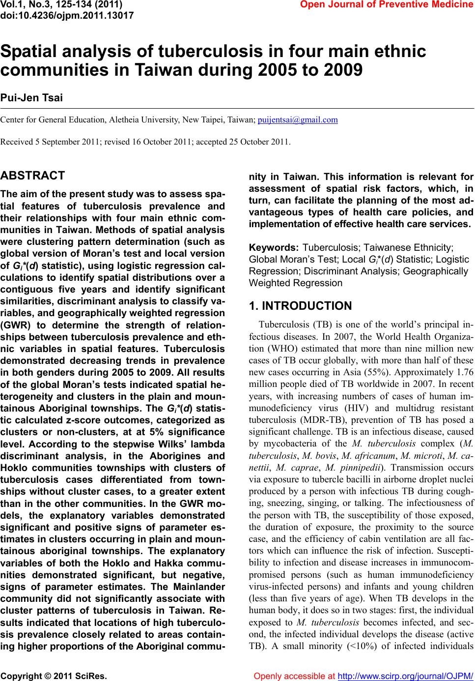